Detailed Analysis

In this section, we aimed to deepen the analysis of some trajectory of interest. With hierarchical clustering and PCA of the trajectories' RMSD values, we find an interesting behaviour in mt2_rep0. For better understanding this phenomenon, we introduce a specialized version of the contact map analysis, abbreviated DCMD, were we calculate the difference between the contact map of different frames. We observe an interesting result around frame 5500, which we then check in VMD and find out it is caused by the protein "opening up" momentarily. From the evolution in VMD we also noticed that the active site gets "obstructed" near the end of the trajectory.

Unsupervised Clustering

In the general analysis section we calculated the RMSD for the trajectories. The RMSD is only an indicator of the stability of the protein, so considering only this parameter we cannot be sure that system is at equilibrium. To have a better insight of the possible configuration changes we use the hierarchical clustering method. With this procedure we aim to identify clusters for each frame, where each cluster collects the frames particularly near to each other (in terms of RMSD). We set the clustering linkage method as ward and the labelling criterion as distance.

Hierarchical Clustering

We begin the clustering analysis by introducing clusters to the RMSD calculated in the previous section. Hopefully, the points belonging to the same cluster represent configurations geometrically similar to each other. To decide which frames are near it is necessary to introduce a threshold on the difference between two RMSD values. This is given by the t_value of the clustering method. However, in the plot we notice that the points belonging to the same cluster are not necessarily consecutive frames in the trajectory.

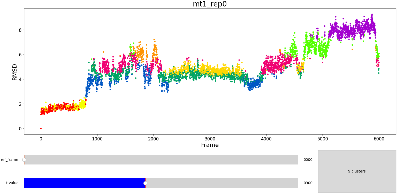
clustering/mt1r0.png — Hierarchical clustering. Clusters are represented by different colors.

Using the same default parameter t_value = 900, the rep0 for the four trajectories was inspected in search for possible interesting clusters. At this value, mt1 gets fragmentated into many clusters, while wt1 and wt2 are so uniform that their clusters are similar and not very insightful. On the other hand, mt2 has a well defined cluster at the end of the trajectory, which gives the impresion that the trajectory might be undergoing a change of conformation near frame 5500.

animations/clusters_1.gif — Clusters for different values of the parameter t are represented. For lower values of t the number of cluster increases.

animations/clusters_2.gif — By highlighting the cluster of the current reference frame, we notice members of the clusters can be in unexpected places. For example, some points belonging to the yellow cluster lie in the first part of the trajectory while the great majority of them are at the end of the trajectory.

Principal Component Analysis (PCA)

The trajectories under study consist in a large number of particles and frames. Dealing with many degrees of freedom is challenging, so dimensionality reduction techniques such as PCA prove to be useful. These allows us to represent the system in a more comprensible way, which helps to understand how the datapoints (in our case, the frames) are distributed. Having said this, we applied PCA to the RMSD values to observe possible clusters in this other way.

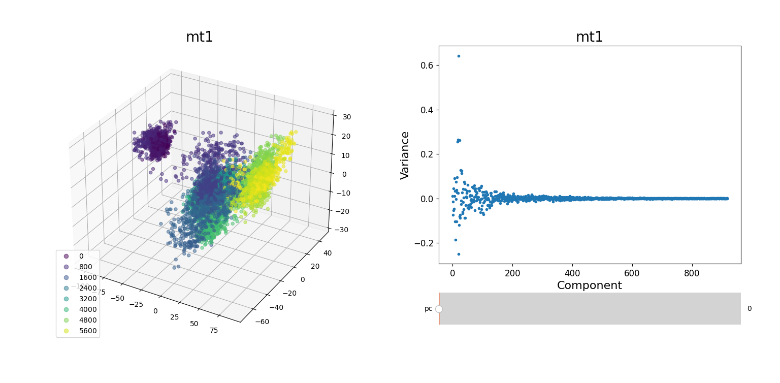
pca/mt1.png — PCA. Left) Frames projected on the 3 principal components. Right) Covariance between the components.

In the plots to the left, clusters for the trajectory under study can be found by projecting their frames into the most important components. In some cases a distinct separation of some data points is evident, namely mt1 and mt2. The plots on the right represent the covariance between the components. Similar to other dynamic plots presented before, a single row of the covariance matrix can be observed at a time by using the slider.

As hierarchical clustering showed that mt2 has an interesting clustering, we focus on how the frames of this trajectory cluster when performing PCA. Effectively, the frames conforming the cluster of interest for the hierarchical method also have an interesting behavior under PCA. We can observe that most frames cluster together in an ordered manner, representing similarity in their configuration, while frames after 5000 are highly spread.

animations/pca.gif — PCA for mt2. Left) Points corresponding to the final frames behave significantly different under this projection. Right) Each row of the covariance matrix can be examined at a time.

This observation complements hierarchical clustering, by hinting that, even though the final frames can be placed under a same cluster because they differ significantly from the rest, the final frames differ also amongst themselves. This can also be confirmed when observing the animation above for the higlighted clustering plot. We conclude that there might be some sort of transition happening during these frames.

Dynamic Contact Map Differences (DCMD)

We want to investigate the mt2_rep0 trajectory to understand what kind of behaviour it has between frames 5000 and 6000, specifically to test the idea that there might be some sort of conformational change. A reasonable approach would be to compare the contact maps of different frames over this time period, which we can implement by following the same philosophy of adding an additional "interactive" dimension to the plots. This is the principle behind what we call Dynamic Contact Map (DCMAP).

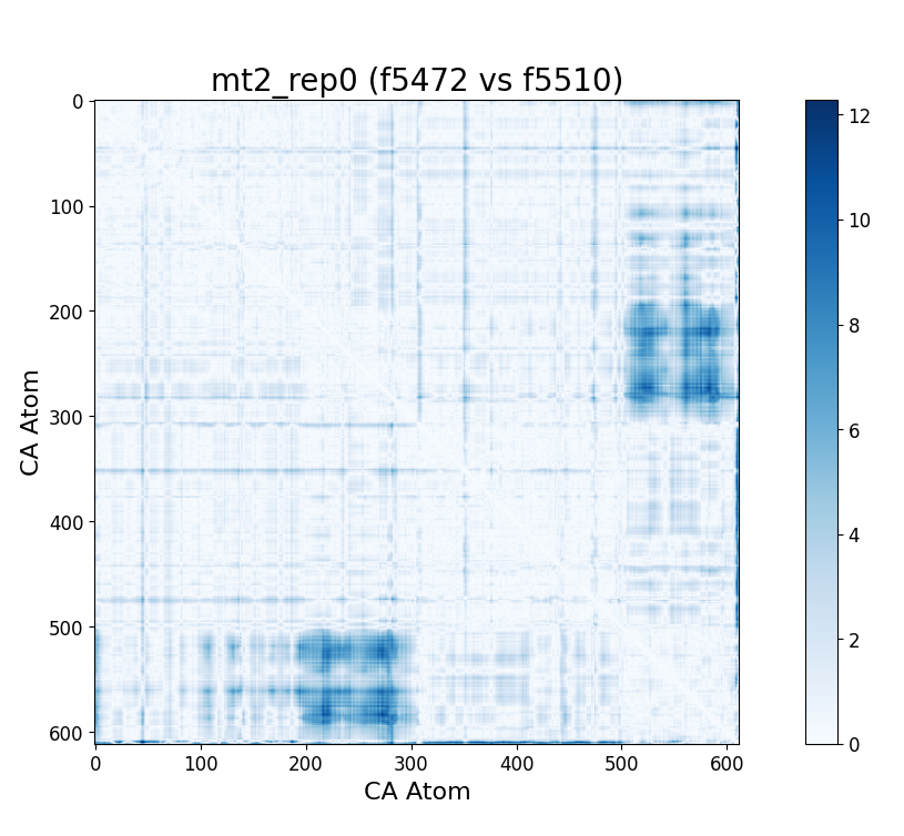
animations/dcmap.gif — DCMAP matrix. Each point represents the distance between residues $i$ and $j$ at a given frame.

We can observe that this is not very insightful, as the patterns from the CMAP matrix are similar throughout the trajectory. However, what we can do is compare the difference between the CMAP at two frames $f0$ and $f1$. The idea is that if there is some conformational change in a specific part of the protein between $f0$ and $f1$, the affected zone will be highlighted in the plot because the difference in its CMAP values will be significant. We refer to this as the Dynamic Contact Map Differences (DCMD) approach.

animations/dcmd_2frames.gif — DCMD matrix. Each point represents the difference of distance between residues $i$ and $j$ at frames $f0$ and $f1$.

After some inspection, we can immediatly spot a high difference in CMAP values for residues 200-300 and 500-600 through several frames. We pinpointed the frame 5510 as the epicenter of this behaviour, having high differences with frames preceding (up to 5472) and succeding (up to 5692) it. Note however that there is no significant CMAP difference between the frames 5472 and 5692 themselves.

cmap/mt2_f5472_f5510.png — CMAP Differences matrices. The frame 5510 is of interest.

In fact, around frame 5510 is where the RMSD values abruptly change and the "final frames" cluster starts, which complements the observations from DCMD. Similarly, if we recall the comparison between RMSF values of mt2 and wt2, we see two very high peaks between residues 289-312 and near 590-600 that are present in mt2 and abscent in wt2, which also concides with some of the residues of interest spotted by DCMD.

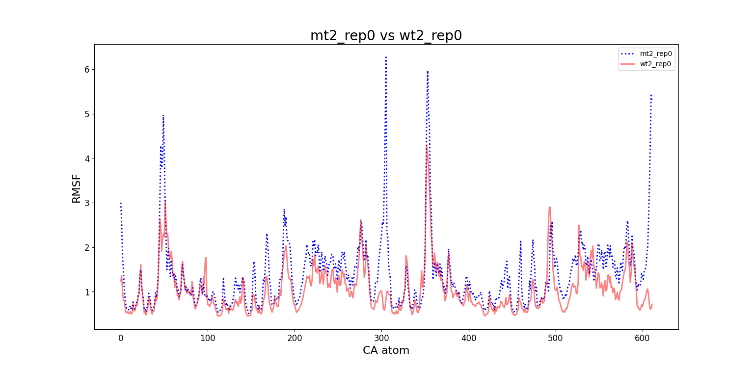
figures/rmsf/mt2_wt2.png — Comparison of RMSF values between `mt2` and `wt2`.

With these evidences, we can infer that a small conformational change starts around frame 5472 and ends around frame 5692, having its most unique configuration near frame 5510. However, the conformations before frame 5472 and after frame 5692 are still somewhat similar, which suggests that this "conformational change" is some sort of temporary unstable transition conformation, that however leaves some repercusion after returning to its more stable configuration (explaining the change in RMSD values).

Furthermore, the residues in the ranges 200-300 and 500-600 are involved, which after considering that each subunit has a size of 306, actually means residues between 200-300 in the first subunit and 200-300 in the second subunit. This could imply that the transitory conformational change involves perhaps some way of symmetry. This effect is specially evident near the ends of the subunits. We confirm these insights by observing directly the trajectory at the time and place of interest.

animations/protein_opening.gif — Behaviour of the trajectory between frames 5000 and 6000. The protein "opens up" momentarily near frame 5500. The subunits are represented in different colors. Residues between 200-300 and 500-600 are displayed in a semi-transparent overlay.

Active Site

Covering of the Active Site

In the previous animation, we can observe that one end of the green subunit is moving around freely, but after the "opening up" event it starts to interact with some residues in the purple subunit. We further explored this interaction, and noticed that the interacting residues of the latter subunit were actually very close to its active site.

animations/AS_observation_1.gif — Behaviour of the trajectory between frames 5000 and 6000, different angle. Orange) Reactive part of the active site. Purple) Surroundings of the active site. Red) Residues 45-50. Yellow) Residues 289-312. Green) Residues 350-356. Blue) Residues 593-612.

By displaying the estimated surface area of the protein, we can actually observe that this interaction seems to cover up the active site. This is a significant observation: if these conformations where the active site is obstructed are stable, they might appear frequently in the long run and imply a hindering in the activity of the active site. Unfortunately, this event happens near the end of the trajectory, so we can not observe how stable it is.

animations/AS_observation_2.gif — Estimated surface of the protein. Reactive atoms from the active site are represented by spheres. They get obstructed at the end of the animation. White) Hydrophobic residues. Green) Polar residues. Red) Negative residues. Blue) Positive residues.

animations/AS_observation_2a.gif — Estimated surface of the protein. The active site is obstructed immediatly after the "opening up" event. White) Hydrophobic residues. Green) Polar residues. Red) Negative residues. Blue) Positive residues.

animations/AS_observation_3.gif — Detailed representation of some residues involved in the "active site obstruction" event. White) Hydrophobic residues. Green) Polar residues. Red) Negative residues. Blue) Positive residues.

Effect on the mutation on Active Site interactions

We were also interested in seeing if the presence of the mutation affected in some way the local interactions in the active site. For doing this, we calculated the contact values of specific atoms and averaged them through all the frames, as a measure of how much they interacted during the simulation. We did this for all repetitions, however we did not observe any evident difference on the behaviour of the trajectories, apart from some outlier points (interactions EG, GH, IJ from wt2_rep1_as0).

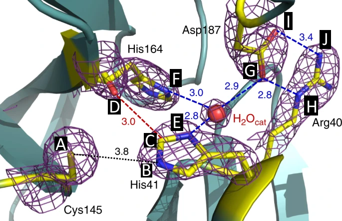
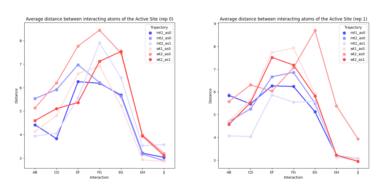
figures/cmap/residues.png — Main interactions between atoms of the active site. Ten atoms are labelled with letters A to J. Adapted from Kneller *et al*.

figures/cmap/AS.png — Average contact between labelled atoms in the active site. For systems with two subunits, a data point is obtained for each subunit, identified here with the suffix `as0` or `as1` respectively. Left) `rep0` for all systems. Right) `rep1` for all systems.

Pyinteraph

We wondered if there are some correlations between the "opening up" and "active site obstruction" events described before. In particular we wanted to further explore what kind of interaction occurs between the residues involved. For adressing this, we briefly refered to Pyinteraph, a software designed to identify interaction networks. We followed the Pyinteraph workflow to obtain interaction matrices between residues during the met2_rep0 trajectory.

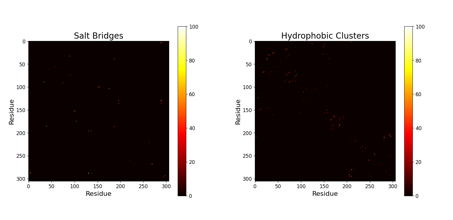
This plot portrays the salt bridges and the hydrophobic interactions between couples of residues. Two hydrophobic residues interact if the center of mass of the side chain of the two residues is found within 5 Å. Two charged groups interact (salt bridges) if their distance is less than 2.5 Å. In this case the distance between residues is computed as the shortest distance between two of their atoms. Evidently, the interaction matrix for hydrophobic clusters is more populated, as the minimum distance treshold is double than that of salt bridges.

A deeper analysis could be performed using Pyinteraph for frames before and after the "opening up" event in an independent way. Comparing the interaction maps of such results could prove insightful, however we do not include it in this work.

To exemplify this idea, some possible results obtained by this approach can be searched manually. By taking the interactions with higher occurance that however do not equal $100\%$, some of these could be residues that were always interacting but got disrupted during the trajectoy.

In fact, one of the salt bridge interactions with higher occurance ($88.4\%$) happens between residues 5 and 290. Residue 290 is in fact in the range of residues of interest described previously, and when checking the trajectory, this interaction is indeed strongly present throughout the frames until the "opening up" event, where it gets disrupted permanently.