General Analysis
The source code for the general, detailed and solvent analysis is found in the folder src_analysis/. It contains scripts for both calculation and visualization of the results, which are to be accessed using the src_analysis/main.py script. Numerical results are stored in a folder created while executing src_md/3_POST.sh, called data_analysis/.
Calculations
Calculating the different methodologies below can get computationally expensive when dealing with a trajectory of $6000$ frames. For example, the RMSD matrix would consist of $6000 \times 6000$ elements. Firstly, one must consider that large XTC files should be opened as a stream (loading just the frame needed for a given operation) instead of loading all frames in memory. This means that, when calculating the RMSD matrix, the XTC "reading window" must shift from start to finish multiple times to load the required frames, which is highly demanding.
Considering this, the function calculations.extract_ca_coords was defined. It iterates over the XTC once, assigning the coordinates of the backbone carbon alpha atoms for each frame into a numpy array, then saving the whole array in data_analysis/_coords/*.npy. This data structure is much lighter and can be loaded into memory for any method that requires using the backbone positions of the protein.
Furthermore, as the RMSD matrix is symmetric, the function calculations.calc_rmsd calculates only half of the matrix, and then assigns the other half in a specular manner. This structure is also stored in data_analysis/rmsd/, to avoid calculating the RMSD each time a different visualization is performed. This idea of pre-calculation is also applied for other subsequent analysis methodologies, always using the same numpy-friendly NPY binary format.
Ramachandran Map (RAMA)
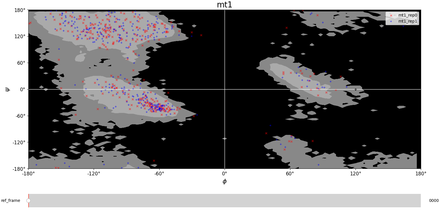
We compare the theoretical Ramachandran map with the experimental one to check if the protein assumes allowed configurations during its evolution. From the plots below we notice that the great majority of the points falls into the gray region, meaning that the protein assumes allowed configurations. Few points fall in the black region, but this could correspond to unstable configurations, in which the protein is moving to a more stable configuration.
Root Mean Square Deviation (RMSD)
From the trajectories visualized in VMD it can be seen how the protein fluctuates during its evolution in water. The first frame, which is the PDB file taken from crystallographic experiments, represents the protein in a structure far from equilibrium. During its evolution, the system should move towards a minimum of the free energy, and reach more stable configurations. We wonder if the system reaches an equilibrium configuration, and if there are some transitions from a metastable configuration to another. To explore this behaviour we can calculate the root mean square deviation (RMSD) for each trajectory. The RMSD between two frames is defined as $$RMSD(\Delta t) = \sqrt{\frac{1}{N}\sum_{i=1}^{N}(x_{i}(\Delta t)-x_{i}(0))^{2}}$$ where
- $N$ is the number of atoms in the protein
- $\Delta t$ is the time step
- $x_{i}(\Delta t)$ is the position of atom $i$ at time $\Delta t$
RMSD visualization - 1D
A frame from the trajectory can be taken as a reference point for the RMSD with other frames, as a means of general comparison between conformations and their evolution. By taking the respective row from the RMSD matrix, a fixed 1D representation can be obtained. The classes visualizations.Plotter_RMSD_1D and visualizations.Plotter_RMSD_1D_Compare were defined with this purpose in mind (the latter allows for plotting two RMSD lines simultaneously).
In the following plots, the RMSD is visualized with respect to the initial frame, to estimate if the proteins reach an equilibrium during the evolution of the system (i.e. a plateau on RMSD values with respect to the original structure). Furthermore, each plot contains both simulation repetitions, which allows to directly compare them. In general, the noise is quite high, and it is not straightforward to identify the stable or equilibrium regions on the plots.
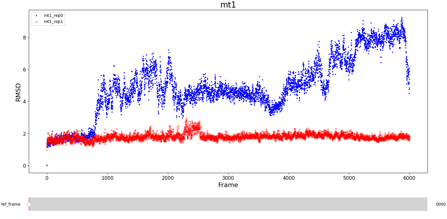
MT1
The first system, mt1, presents large differences in their RMSD values. An important disturbance seems to occur around frame 900 for rep0 (but not for rep1) and a change in the trend of configurations can be noticed. Always in rep0 we observe an equilibrium region approximately between frame 2100 and frame 3800. However, before frame 2000 an extremely noisy region occurs, and after frame 4000 it seems that the configuration of the protein changes. Meanwhile, in rep1 the RMSD fluctuates around a constant value and is much less noisy than the rep0 one. The only relevant change occurs between frame 2000 and frame 3000, which might be a slight conformational change.
WT1
The RMSD of rep0 is quite low and it seems to oscillate around a constant value. It seems that no major changes of configuration occur. On the other side, the RMSD of rep1 undergoes several changes. At frame 800 it changes abruptly, perhaps consequence of a similar disturbance as suffered by mt1_rep0. Until frame 4000 it seems that the protein stays in the same equilibrium configuration, only to then present extreme changes on the RMSD values.
Overall, the systems with only one subunit seems to be highly unstable, sometimes apparently reaching equilibrium quickly while other times undergoing extreme changes because of slight perturbations. This is most likely related to the fact that this systems do not appear in nature, as the protein is expected to be constituted by two monomers. Perhaps this is so because having two monomers provides structural stability to the polypeptides, and could explain why this is the form found in nature. Effectively, when checking the evolution of the dimeric systems (wt2, mt2), a higher stability is observed.
MT2 and WT2
It is noticeable how stable the wt2 system is with respect to the other trajectories. However, this should not be a surprise, as this system is the wild-type dimeric form prevalent in nature. The mt2 system is also quite stable, with seemingly only one relevant conformational change in both runs, between frame 4000 and 6000.
Dynamic RMSD 1D
All classes inherited by visualizations.Plotter_RMSD_1D also allow to "slide" the reference frame in an interactive manner. This allows for a better understanding of the whole RMSD matrix, as exemplified bellow.
RMSD visualization - 2D
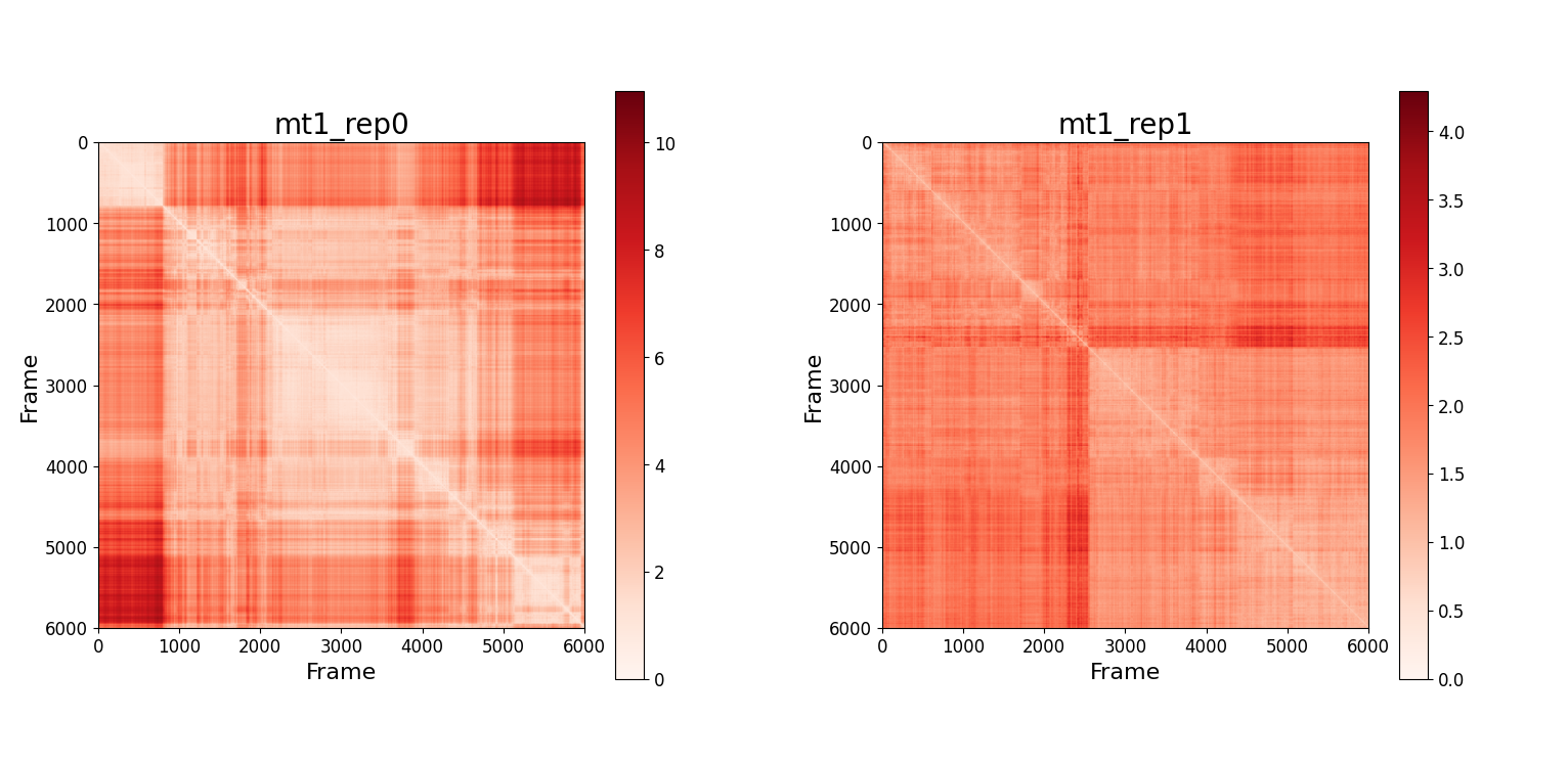
It is also possible to represent the RMSD matrix using a heatmap. Recalling that the static RMSD plots presented in the previous section correspond to the first row in the respective matrix, this plotting method can give a broader idea of the behaviour of the system. These matrices are symmetric, and the values on the diagonal are $0$ (by definition).
-
MT1: It seems there is a change in configuration in
rep0around frame 800. Other changes in configuration occur but the contrast is lower. Inrep1map the contrast is much lower, meaning that the protein does not undergo major changes in its configurations. It is interesting to observe that two changes in the protein structure occur around frame 2500. In the fixed 1D plot we could not grasp this information. -
MT2: In
rep0only a change in the configuration occurs around frame 5500. Inrep1several changes occurs, and the value of RMSD is in general higher than the ones inrep0. -
WT1: Here we observe two deeply different behaviours in the RMSD. In
rep0the values are substantially constant and it seems that no important changes in the configuration occur. Inrep1a clear change in the configuration occurs around frame 4000. -
WT2: The RMSD values in both repetitions seems to be similar. In
rep1a change in conformation seems to occur around frame 3000.
Difference between repetitions for single-subunit trajectories
We noticed that the RMSD matrices of rep0 and rep1 behaved in a highly different way. We think that this happens because the system has not equilibrated in the $300 ns$ of simulation time. This effect is more evident for mt1 and wt1, which may be due to the fact that the protein consists of two subunits in nature. The systems with one subunit are artificial and might be more unstable. This explain why the protein requires two identical subunits.
The initial velocities are different for the two repetitions of the same simulation since they are randomly taken from a Maxwell-Boltzmann distribution at fixed temperature. We also noticed that after the energy minimisation step the positions of the heavy atoms change and the same happens after the following steps (NVT, NPT equilibration). Perhaps these small deviations in the initial conditions (GRO file used for the unrestrained MD) influence the trajectory in a significant way, specially for the systems with one subunit.
Root Mean Square Fluctuations (RMSF)
The protein is composed of many atoms which move during the evolution of the system. To understand which parts of the protein are more mobile it is useful to calculate the root mean square fluctuations (RMSF) for each atom. The RMSF related to atom $i$ is defined as: $$ RMSF_{i} = \sqrt{<\Delta \vec{r_{i}^{2}}>} $$ where $<\Delta \vec{r_{i}^{2}}>$ is the mean deviation of the atom from its equilibrium position.
For better understanding the behaviour of the RMSD values, we can observe the RMSF for their trajectories. In the plots below, whenever an atom has a larger RMSF, they are more mobile during the evolution of the protein.
Comparing repetitions of the same system
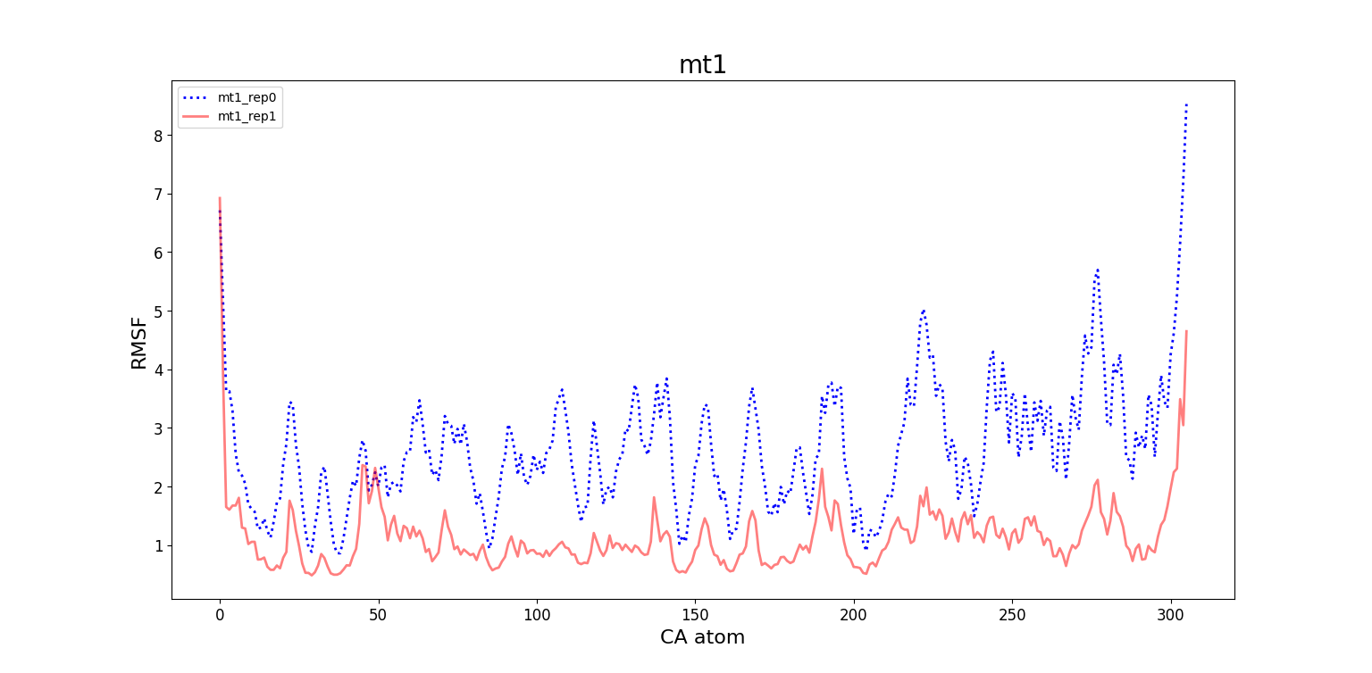
For mt1 and wt1, the RMSF values differ significantly between rep0 and rep1, which is compatible with the high difference between the RMSD matrices of said systems. Futhermore, the high variations on the RMSD map for wt1_rep1 can be explained by the large values of RMSF of its residues, specially near the terminal 306. On the other hand, RMSF values between rep0 and rep1 for mt2 and wt2 are more similar, reflecting the similarity between their RMSD matrices.
Comparing different systems
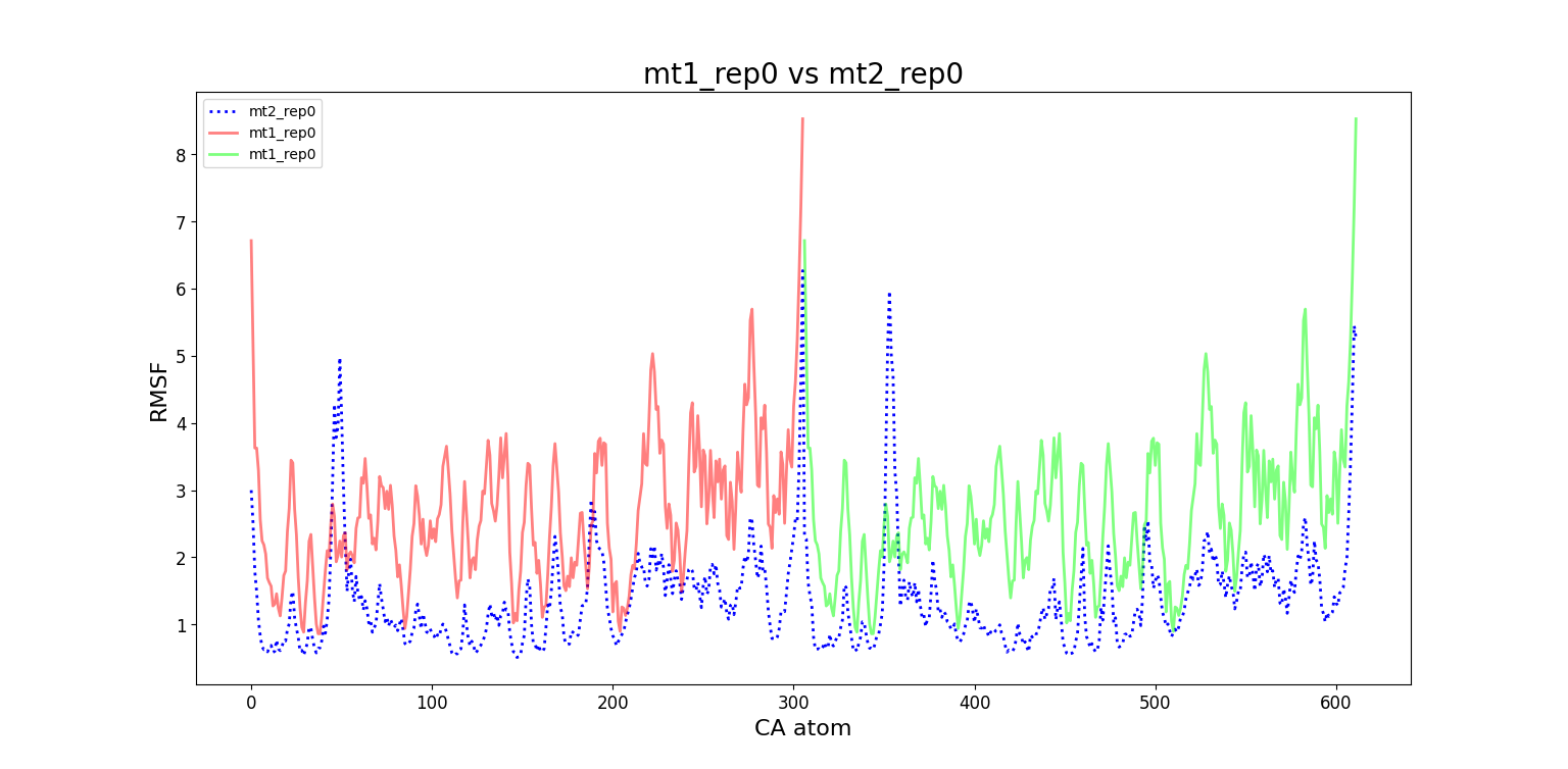
Here we compare the RMSF of the whole protein with the one computed for only a subunit. In this way we can explore how the fluctuations of atoms in a given subunit are correlated to the fluctuations in the other subunit. We also observe that when the mutation is introduced to a single subunit, it becomes more unstable (higher RMSF values). However, when grouping the subunits in a dimeric form, both wt2 and mt2 reach a similar stability. This reaffirms the idea that these subunits are more stable when they are in a dimeric complex, as is the case of 8DFN and 7SI9 in their natural state.
Radius of Gyration (RGYR)
From VMD it can be observed that even though the protein fluctuates, its shape remains constant. To check if the protein "elongates" during its evolution it is useful to calculate the radius of gyration: $$ RGYR(\Delta t) = \sqrt{\frac{\sum_{i=1}^{N}m_{i}(r_{i}(\Delta t)-R_{cm})^{2}}{\sum_{i=1}^{N} m_{i}}}$$ where
- $m_{i}$ is the mass of atom $i$
- $r_{i}$ is the position of atom $i$ at time $\Delta t$
- $R_{cm}$ is the center of mass
For better understanding what kind of fluctuations are represented by RMSF, we can observe the Radius of Gyration (RGYR) for the trajectories. In the plots below, whenever a frame has a larger RGYR, we think that some residues might be "unwrapping" and moving around with more liberty, which implies a larger RMSF value for those residues.
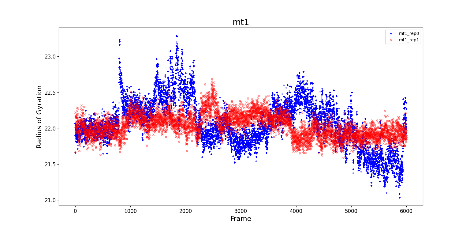
In the following plots we present the radii of gyration for the four systems. There is a significant amount of noise, so few assumptions can be done as regard the compatibility between the two sets of data and the configurational changes of the protein. The RMSF computed for rep0 and rep1 seem to agree more for mt2 and wt2, i.e. for the evolution for the whole protein. This could mean that a single subunit is less stable than two subunits linked together.
-
MT1: The radius of gyration, RGYR, for
rep0presents a peak around frame 900, and two local maxima around frame 2000 and frame 4000. A non constant RGYR could mean that the protein is changing shape, i.e. it is compatible with a change of the configuration. The RGYR forrep1oscillates around $220nm$ and it slightly increases between frame 1000 and frame 3800. In this interval it is possible that a conformational change occurs. -
MT2: The values of the RGYR are extremely noisy, so it is quite difficult to understand if a change of conformation occurs. In
rep1a peak is observed around frame 4800, and inrep0the same peak occurs around frame 5500. We think that the protein assumes similar configurations around frame 4800 and 5500. - WT1: The RGYR of the two repetitions quite agree, it seems they both evolve with a sinusoidal trend.
-
WT2: The RMSD values in both repetitions seems to be similar. In
rep1a change in conformation seems to occur around frame 3000.
Contact Map (CMAP)
The protein is constituted by a folded chain composed of atoms linked together. Non subsequent atoms can be near enough to interact even if they are not adjacent. We can observe the distance between two atoms for having an idea on whether they interact with each other. The contact maps (CMAPs) show the distance between atoms for a single frame.
Here we show as an example the contact maps calculated at the initial frame of the trajectory. The contact maps at the initial frames for both repetitions of wt1 and mt1 are almost identical because the structure is basically the same. Intuitively the upper left and lower right quadrants of the contact map of the wt2 and mt2 are very similar to their monomeric counterparts.
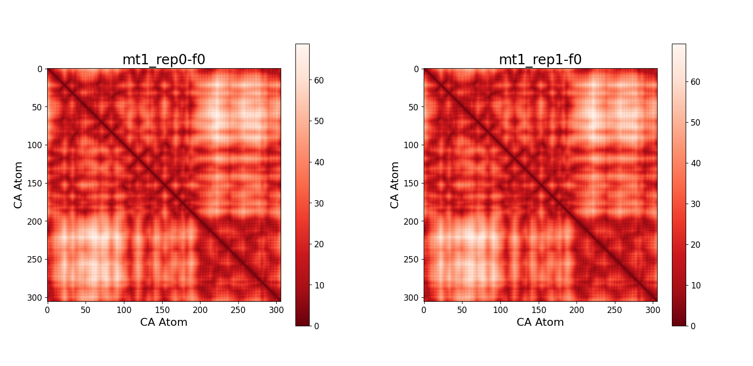
The darkest parts represent the regions in which there is more contact between the residues, while the brightest parts correspond to the regions in which there is less contact. In the contact maps for systems with two subunits, a discontinuous line indicates the region in which the first subunit ends and the second one begins. It is also evident that the map is symmetric, as distances are symmetric by definition. Some secondary structures can be inferred by observing the lines tangent to the main diagonal, namely antiparallel $\beta$ sheets.
Block Analysis (BSE)
During this first part of the analysis we sought to understand whether the system has reached equilibrium during the simulation, but the variables we observed only gave us some indications. Looking at the RMSD, one of the most important indicators of equilibrium, we noticed that its values had an approximately constant trend toward the end even if many fluctuations were present.
Block Averaging Analysis method
The Block Averaging Analysis is an elegant method to estimate the autocorrelation time $\tau_f$. A trajectory with $N = M \times n$ snapshots is divided into $M$ segments of length $n$ with $n =1, 2, \dots$. For each block we can compute the average
$$\langle f\rangle_i, \qquad i = 1, \dots, M$$
and the standard deviation $\sigma_n$ for each value of $n$. The running estimate of the overall standard error is defined as
$$BSE(f, n) = \frac{\sigma_n}{\sqrt{M}}.$$
For small values of $n$ and high values of $M$, the Block Standard Error (BSE) under-estimates the statistical error, because we are assuming that all data points are linearly independent when in fact they are not. The $BSE$ reaches a plateau (does not depend on $n$ anymore) once the blocks are independent of one another, which means that we have included in a block a number of snapshot which correspond to a time equal or grater than the autocorrelation time. At this point it does not matter anymore how the system is subdivided into blocks. Once the correlation time, or the correspondent frame has been estimated, it is possible to calculate the number of independent values of the RMSD as
$$N_{RMSD}^{ind}\simeq\frac{F_{sim}}{F_{corr}}$$
where $F_{sim}=6000$ is the total number of frames in the simulation and $F_{corr}$ is the frame at which the BSE reaches a plateau.
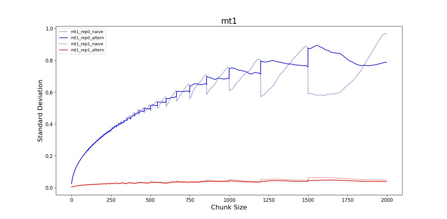
- MT1: The frame for which BSE seems to reach the plateau is $F_{corr0} =1000$ for
rep0and $F_{corr1} = 200$ forrep1. In this last case we observe that the BSE forrep1appears as a constant line and we could not precisely estimate $F_{corr1}$. The number of independent RMSD values is $6$ values forrep0and $30$ values forrep1. - WT1: The frame for which BSE seems to reach the plateau is $F_{corr0} =200$ for
rep0and $F_{corr1} = 1000$ forrep1. In this last case we observe that the BSE forrep0appears as a constant line and we could not precisely estimate $F_{corr0}$. The number of independent RMSD values is $30$ values forrep0and $6$ values forrep1. - MT2: The frame for which BSE seems to reach the plateau is $F_{corr0} =750$ for
rep0and $F_{corr1} = 1250$ forrep1. The number of independent RMSD values is $8$ values forrep0and $5$ values forrep1. - WT2: The frame for which BSE seems to reach the plateau is $F_{corr0} =1000$ for
rep0and $F_{corr1} = 750$ forrep1. The number of independent RMSD values is $6$ values forrep0and $8$ values forrep1.