Solvent Analysis

In the first part of this section we present a brief introduction on water models, in particular the TIP3P model that was employed in our simulation. Then, we introduce a new methodology for analyzing the water distribution around the protein, called WALD. Finally we estimate the accessible surface area with the GROMACS tool SASA.

Water Model

Modelling water is a challenging task and many different models are available. The choice of the water model is determined by

The size of the system.
The simulation period.
The physical properties that have to be simulated with the most accuracy.

The most suitable model for our system was the TIP3P, This water model is widely used because it is not too computationally demanding. Even to simulate a simple protein in water, a large number of water molecule is required, and their positions and velocities have to be updated at every time step. It is then necessary to have a quite simple water model. More complex models are available, but it is possible to employ them only on small systems, with less than $1000$ water molecules, and for short simulation periods $(\simeq1ps)$. These are not the length and time scales of biophysical systems.

This model, as many other frequently used, ignores the proton hopping from one molecule to another, which favours the cluster formation. It describes the water as a planar molecule, with three interaction sites, an oxygen atom and two hydrogens. the atoms interact due to the coulomb interaction and are modeled as point like particles. the long range electrostatic interaction is truncated after a cutoff distance. the oxygen atom also interacts with other molecules by means of the Lennard-Jones interaction. Source.

Water Average Local Densities (WALD)

After the observations regarding the "active site obstruction" event in the previous sections, we are interested in knowing if the accesibility of the active site by its ligand is indeed affected or not. An intuitive approach is to observe how accesible is the active site to water molecules. Water molecules visit this and other cavities during the trajectory, unless they get obstructed in some way. Therefore, we can keep track of the positions of water molecules through the trajectory, and in this way measure a sort of local density which can hint on the accesibility of water to different spaces of the protein.

We introduce a methodology based in this idea, called Water Average Local Densities (WALD). It is divided in three main parts: selection of frames of interest, calculation of local densities, and visualization of results. The script src_analysis/wald.py is to be used for executing the different steps of the pipeline. We follow this workflow for mt2_rep0, so for simplicity any file path described will specify this particular run.

Step 0: Frames Selection

The WALD method averages over a set of frames to obtain the average local densities. The final result is displayed as an overlay on top of the protein at a particular frame of interest. Therefore, it is sensitive to select a set of frames that are structurally similar to the reference, in order to have good results. We choose RMSD as a measure of similarity, and choose all the frames of the simulation under a given treshold RMSD value against the reference frame.

To facilitate this procedure, we provide an adapted version of the interactive RMSD plot, where both reference frame and treshold values can be modulated and then saved in data_analysis/wald/mt2_rep0-info.json. This file contains different values and parameters required by the methodology and allows to "communicate" easily between different steps without having to restart all the workflow each time changes are introduced. This step can be executed by using the command wald.py -0.

animations/wald_rmsd.gif — Interactive RMSD. The reference frame and maximum RMSD treshold value can be modulated to manually cluster points that will be the set of frames for the WALD methodology.

Step 1: Local Densities Calculation

The WALD method is a grid based approach, which means we divide the simulation box in smaller and evenly spaced cubes. A three-dimensional grid is then populated with the experimental density values of these cubes (hence the name local densities). The size of the grid is a relevant parameter, too few or too many points would lead to pointless results. In our implementation, this is controlled by the parameter WALD_DIVISIONS at src_analysis/wald_pipeline/_params.py. We found that WALD_DIVISIONS = 20 is a good empirical value for the parameter, which means that WALD grids will have a shape of $20 \times 20 \times 20$ and a size of $8000$.

Populating the WALD grid is straightforward. For each grid point, we count how many water molecules go into its respective grid for all the frames of interest, then divide it by the number of frames of interest to obtain the average. This step can be executed by using the command wald.py -1.

Visualization

Visualization of the results is trickier, as we would like to represent the three-dimensional grid together with the protein in a non obstructive way. We had to choose between implementing a 3D mesh semi-transparent display method on a molecular visualization tool (such as VMD) or to implement a protein display method on a standard plotting library (such as Matplotlib or Plotly). We chose the latter (namely using Plotly) to keep the overall implementation on the same Python workframe. However, some usage of VMD is still required, as will be presented now.

Step 2: Preparation of meshes with VMD

We need to somehow export a visual representation of the protein as a 3D "image" that can be parsed by the WALD pipeline. Luckily, VMD provides a rendering option that includes the OBJ/MTL standard, so we will work with that. Without getting much into the details, the most appropriate representation for the system is the Quick Surface of just the protein, as it is informative and requires relatively few vertices and faces to be rendered (hence plotting it is more efficient).

This step can be executed by using the command wald.py -2. A TCL script will be automatically generated as data_analysis/wald/mt2_rep0.vmd. This has to be opened with VMD for exporting the meshes before proceeding to step 3. An explanation on how to do this is provided by the manual of WALD, accesible by wald.py -h.

Step 3: Conversion of meshes

Unfortunately, OBJ/MTL files are not directly supported by Plotly, so we have to parse them into a a custom format that is more compatible with the plotting library. We will not explain much this process because it is outside of the scope of this report. In summary, OBJ/MTL are text-based formats, which we parse using Regular Expressions and finally export the data into the usual NPY binary format.

Note that due to the complex nature of the parsing and the many ways VMD has to optimize their rendered OBJ/MTL files, this is a critical step that can go wrong if the preparation with VMD is not done correctly. We plan to improve this pipeline in the future for a more robust solution. This step can be executed by using the command wald.py -3.

Step 4: Display of results

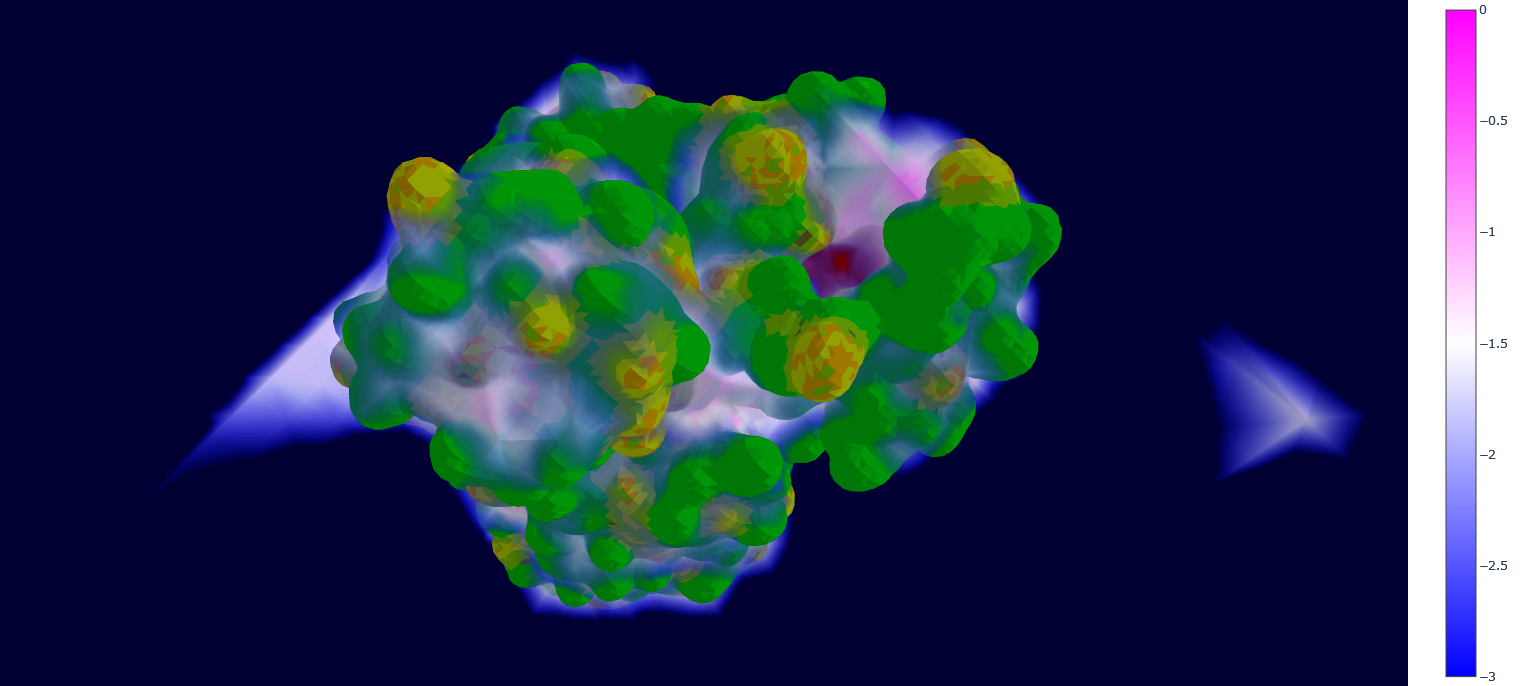
We finally have the local densities matrix (wald/mt2_rep0-wald.npy) and the protein mesh data (all the other wald/*.npy files), now we just have to display them with Plotly. An intuitive approach when plotting 3D grid data on top of a solid object is to use semi-transparent colors for the data points, where higher values are more opaque and have a different hue, to mimic the "density" concept represented by the points.

However, it can be quickly noted that here this would generate a thick "cloud" of points around the protein, because it is surrounded by multiple layers of points with very high values of local water densities (due to never being occupied by the protein). To overcome this problem, WALD actually plots the inverse local densities, which are obtained by just inverting the sign of the values and imposing a treshold of minimum and maximum values (points are only displayed if they are inside this range).

As a quick note, one would think that just implementing the tresholds is enough for having useful results. However, inverting the densities gives a gradient of transparency that starts from the protein (less occupied by water) and goes outwards until reaching the treshold, which avoids the ofuscation of points closer to the protein and gives a more insightful visualization. This step can be executed by using the command wald.py -4.

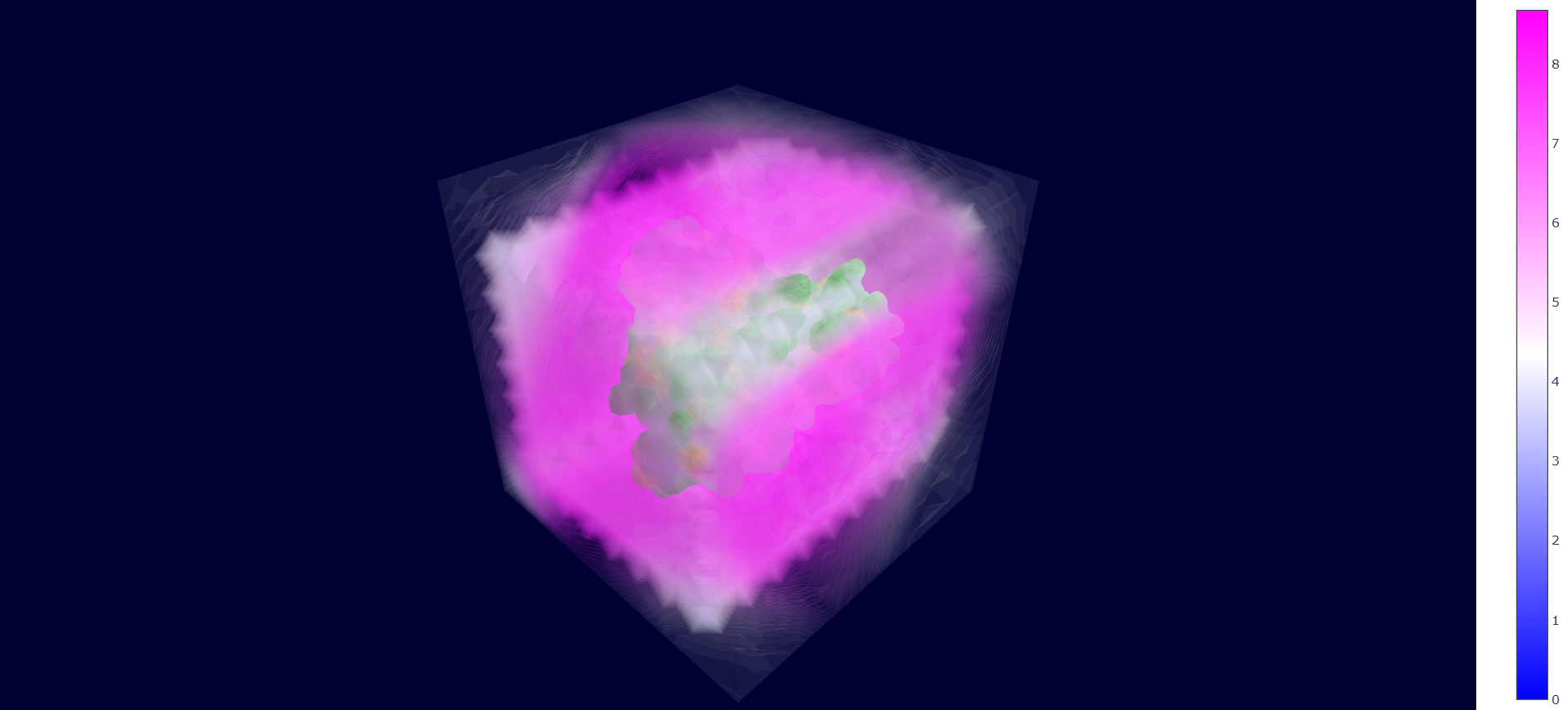
figures/wald/wald_naive.png — WALD grid displayed over the protein. Displaying the thresholded inverse of the grid is more insightful. Color schema for the protein: green) hydrophilic residues, yellow) hydrophobic residues, red) active site. Opaque magenta points represent low water occupancy. Points at the protein surface grade towards more transparent shades of blue that represent higher water occupancies.

animations/wald_result.gif — The protein and WALD meshgrids can be moved around interactively.

As mentioned at the beginning of this section, we followed the WALD pipeline for reference frames 0 and 5825 of the mt2_rep0 trajectoy, which represent the common available state and the obstructed state of the active site respectively. We observe that at frames conformationally related to 5825 the active site is indeed less occupied by water molecules, confirming our previous observations. Note however that this result is mostly qualitative (we do have the local density values, but we are just visualizing them).

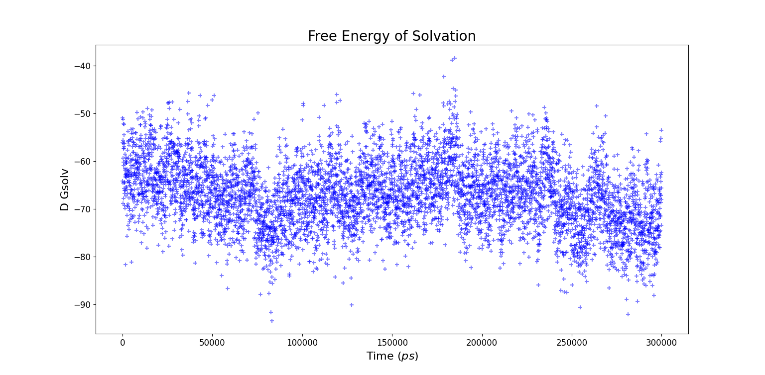
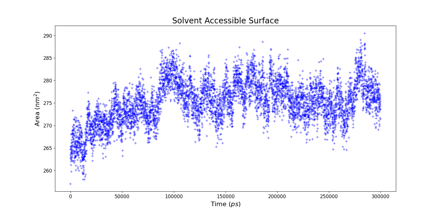
figures/wald/wald_0000.png — Comparison between water occupancy at the active site between frames 0 and 5825.

Solvent Accessible Surface Area (SASA)

A quantitative way to investigate the distribution of water molecules around the whole protein consists in using SASA, a GROMACS tool which computes the solvent accessible surface area. The input file consists in all the non solvent atoms, i.e. the entire protein. Starting from this input the entire surface of the protein is calculated.

figures/sasa/sfe.png — Solvation Free Energy.

The solvation free energy is calculated according to the interaction between water molecules and the external residues of the protein at a given time. It is highly noisy, probably due to the water molecules moving quickly each frame and sometimes being closer to hydrophilic or hydrophobic segments of the protein. The solvent accessible surface area calculated next is derived from this solvation free energy.

figures/sasa/area.png — Surface area accessible by the solvent for each frame.

Using SASA, the surface of the protein which is accessible by the solvent for each frame was estimated. It seems that the area is increasing until $100000 ps$ and then it oscillates around a constant value. The noise is again significant, which difficults infering whether the data follows any trend.

figures/sasa/oa.png — Average surface area accessible by the solvent for each atom over the trajectory.

The aforementioned noise is especially significant in this the case. However, we can observe four atoms with an average surface area of above $0.4 nm^2$ (atoms 704, 705, 5383, 5384). All four atoms correspond to terminal oxygens for glutamine groups. This aminoacid is large and very hydrophilic, so it makes sense that they tend to be in the exterior in contact with water.

figures/sasa/or.png — Average surface area accessible by the solvent for each residue over the trajectory.

A similar behaviour can be seen in the area per residue over the trajectory. We observe that there are two residues with an average surface area higher than $2 nm^2$, namely residues $222$ and $154$. These correspond to arginine and tyrosine respectively, which are again large and hydrophilic groups, with the difference that their overall polar area is even higher than glutamine, which explains why these points overcome the glutamine residues observed before.

figures/sasa/volume.png — Left) Volume enclosed by the surface area in each frame. Right) Their respective density. Similarly to the previous cases, they are very noisy, so we can not make any assumptions on the trend.