Interactive Graph Cut Image Segmentation
Project report for the course Signal, Image and Video, University of TrentoBy Diego Barquero Morera
Introduction
Interactive image segmentation techniques are a promising alternative to fully automatic segmentation. They take a small human input as ground truth and then expand it via an algorithm to segment the image with (hopefully) more realistic and useful results.
For this project, the method described in [1] and [2] was implemented in Python (available here). The goal of this method is to segment a 2D image into two parts (binary segmentation): object and background. A user provides a set of pixels that are certain to be part of the object, and another set of pixels certain to be part of the background. Both sets are denominated seeds for object and background respectively.
Taking into account both sets of seeds, the image is first represented as a directed graph. Then, the image is segmented by finding the optimal cut of the edges of the graph, by exploiting the max-flow min-cut theorem. In the next sections, a brief introduction of these concepts is presented, as well as the details of the algorithm and the Python implementation.
Theoretical Background
Graphs
A graph $G = \langle V, E \rangle$ is defined as a set of nodes $V$ and a set of edges $E$. Each edge $e \in E$ connects a pair of nodes $p, q \in V$, and is represented as $e = (p, q)$. A graph is undirected if $$e = (p, q) = (q, p) \quad \forall e \in E; p, q \in V$$ and directed if $$e = (p, q) \neq (q, p)$$ Finally, in a weighted (or capacitated) graph, each edge $e \in E$ is assigned a weight (or cost) $w_e \in \mathbb{R}$.
An image can be represented as a graph by taking the intensity $Ip$ of each pixel $p$ and assigning it to a node in the subset $P \subset V$. The position information of the pixels is conserved by defining a subset of edges $E_n \subset E$ such that any pair of nodes $p, q \in V$ corresponding to neighbouring pixels in the image is connected by an edge $e_n = (p, q) \in E_n$. Depending on the application, the graph may be defined as undirected or directed; in the latter case, another edge is defined for each pair of pixels $e_n' = (q, p)$. The edges from $E_n$ are known as neighbouring or non-terminal edges. For this implementation, 4-connected pixels are considered as neighbours, although some adjustments can be done for using other criteria.
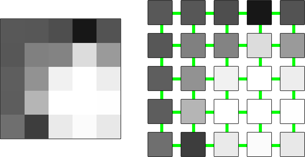
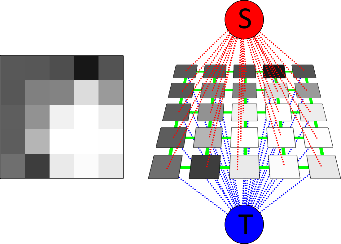
For this segmentation method, two special nodes are added: an "object" terminal called source ($S$) and a "background" terminal called sink ($T$). This means that $$V = P \cup \{S, T\}$$ Furthermore, additional edges connect each node from $P$ to both $S$ and $T$, such that $$E_t = \bigcup_{p \in P} \{(S,p), (p,T)\} \\ E = E_n \cup E_t$$ Note that if directed edges are been employed, the order of the edges from $E_t$ matters.
Graph Cuts
Given a set of nodes $A = \{a_1, \dots, a_n\}$, a path is a sequence of edges that allows to traverse from $a_1$ to $a_n$. A path that starts in the source and finishes at the sink will be denominated here as $path_{St}$. A generic path can be defined as $$Path = \bigcup_i^{n-1} \{a_i, a_{i+1}\}$$ A cut is a subset of edges $C \subset E$ such that in the graph $G' = \langle V, E \backslash C \rangle$ there is no path between the terminal nodes $S$ and $T$. Alternatively, it can be seen as the graph being separated into two sub-graphs, where all the nodes from a given subgraph are only connected to the same terminal node $$ G' = G_S \cup G_T \\ G_S = \langle V_S, E_n' \bigcup_{p \in P_S} \{(S,p)\} \rangle \\ G_T = \langle V_T, E_n'' \bigcup_{p \in P_T} \{(p,T)\} \rangle $$ Finally, the cost of the cut is defined as the sum of the weights of the edges it comprises $$|C| = \sum_{e \in C} w_e$$
Graph Flow
A weighted graph can be interpreted as a network of "pipes" described by its edges, where water can be imagined to flow in a given direction. For the specific graphs described before, the flow starts at the source node $S$, goes through the image nodes $P$ and end up in the sink node $T$ (hence the terminology used for the terminal nodes).
The weights of the edges can represent different concepts under this interpretation, depending on what is required:
- Flow ($flow \ge 0$): The amount of water currently pushed through an edge.
- Capacity ($cap \ge 0$): How much water is supported by an edge. This value remains constant.
- Residual capacity ($res \ge 0$): The capacity left after pushing a certain amount of flow through the edge, given by $res = cap - flow$.
Note the at any given moment the flow going through an edge can't exceed its capacity, so $flow \le cap \implies res \ge 0$. In the specific case when $flow = cap \implies res = 0$, it is said that the edge is saturated, meaning that it is moving the maximum amount of water it can handle. Similarly, a saturated path is a path where one or more edges are saturated. For the purposes of this method, all edges composing a cut must be saturated.
Optimal Cut
The idea of defining all of these concepts is to find a way to quantitatively measure a given image segmentation. Such measure is to be optimized via an automatic algorithm, in order to choose the best image segmentation from the space of all possible segmentations.
Intuitively, a graph cut can be interpreted as the segmentation of the image represented by the graph. An optimal segmentation would be a cut $C$ such that the nodes from the subgraphs obtained, $N_S$ and $N_T$, correspond to pixels that most likely belong to the object and background respectively. This optimal cut corresponds to the cut with the lowest cost $|C|$ and is often obtained by minimizing an energy function of the general form $$E(L) = \sum_{p \in P}Rp(Lp) + \sum_{(p,q) \in E_n}Bp(p, q)$$ where $L = \{L_p \in \{obj, bkg\} | p \in P\}$ is the binary labelling of the image, $Rp$ is a regional penalty function and $Bp$ a boundary penalty function.
As the names suggest, $Rp$ penalizes pixels according to the region they are associated with. Here, "region" refers to either the object or the background, so the penalty works by checking how probable is the pixel part of the object or background, given a prior intensity distribution obtained from the data. This prior is built from the seeds provided by the user. On the other hand, $Bp$ penalizes pixels according to their local interaction with neighbouring pixels, by comparing their $Ip$ values with some sort of metric.
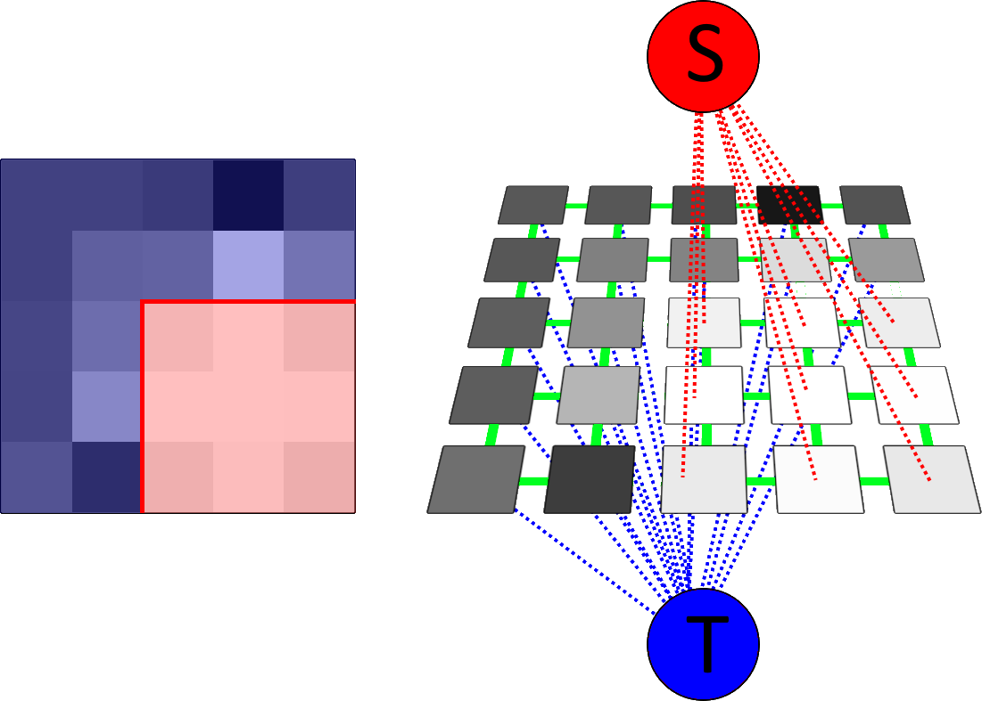
For minimizing the energy and thus obtain the optimal cut, the max-flow min-cut theorem can be exploited. This theorem states that the maximum flow from $S$ to $T$ saturates a set of edges $C^*$ that correspond to the minimum cut, leaving behind two disjoint subgraphs $G_S$ and $G_T$. The objective of many graph based segmentation methods is to take advantage on this duality property and find the maximum flow of the system, which guarantees the minimum cut and therefore the optimal segmentation given the inputs.
Graph Preparation
After mapping the pixels of the image into the nodes and edges of a graph, assigning weights to the edges requires energy functions to be defined. For this implementation, the energy functions were inspired by [1]. Consider $Obj \in P$ the subset of pixels marked as a seed for object and $Bkg \in P$ the pixels marked as a seed for background. Then, the energy functions consist of $$ Bp(p, q) = \exp(-\frac{(Ip - Iq)^2}{2 \sigma^2})\\ Rp_{obj}(p) = -\ln(\Pr(Ip | Obj)) \\ Rp_{bkg}(p) = -\ln(\Pr(Ip | Bkg)) $$ In this implementation, the image is processed as black and white, so $Ip$ is a single value varying from 0 to 1 (the intensities must be normalized for $Bp$ to work correctly). Furthermore, the probability of the intensity given a seed is described by the histogram of intensities for pixels in the given seed. Other approaches could also be considered, such as using the seeds to estimate the parameters of a Gaussian distribution. Additionaly, a constant $K$ is also defined as $$K = 1 + \max_{p \in P} \sum_{q : (p,q) \in E_n} Bp(p,q)$$ The edges can then be assigned weights according to the following table (note that both $\sigma$ and $\lambda$ are parameters that need to be set by the user):
| edge type | weight (cost) | condition |
|---|---|---|
| $(p,q)$ | $Bp(p,q)$ | $(p,q) \in E_n$ |
| $(S,p)$ | $\lambda Rp_{bkg}(p)$ | $p \in P, p \notin Obj \cup Bkg$ |
| $K$ | $p \in Obj$ | |
| $0$ | $p \in Bkg$ | |
| $(p,T)$ | $\lambda Rp_{obj}(p)$ | $p \in P, p \notin Obj \cup Bkg$ |
| $0$ | $p \in Obj$ | |
| $K$ | $p \in Bkg$ |
Taking into account that high cost values are better candidates to be in the minimal cut, it can be noted that $Bp$ returns higher values when $Ip$ and $Iq$ differ significantly, which is a natural way of predicting a border between neighbouring pixels.
Less intuitively, $Rp$ provides lower values when it is more probable that $Ip$ corresponds to the seed. This means $Rp$ is used to assign weights to edges connecting to the terminal of the contrary seed it represents. For example, if a pixel is very probable to be part of "obj", then it should be favourable to cut its edge to $T$ ("bkg"), and so on.
Pixels that are marked as seeds take this to the extreme, by assigning $0$ to their opposite seed, cutting the edge by default since the very beginning. On the contrary, a very high constant $K$ is assigned to the weight of their corresponding seed, making the cut unfeasible under all circumstances. This could also be adjusted to $K = \infty$ if desired.
Boykov-Kolmogorov Algorithm
Motivation
Once the graph is initialized, different algorithms can be used to find the max-flow. For this implementation, an augmenting path based algorithm described in [2] was employed, which will continue to be described as the BK algorithm.
Traditionally, augmenting path algorithms iteratively look for the shortest paths from the source to the sink ($path_{ST}$), having to start the search process each time that all the paths of a given length are exhausted (i.e. they become saturated). The BK algorithm seeks to improve performance of other push-relabel methods by optimizing the step where $path_{ST}$ is searched, by reusing paths from previous iterations.
The basic idea is to build two separate non-overlapping search trees, one starting from $S$ and the other from $T$. These trees are grown (via, for example, breadth first search), and whenever they touch, a $path_{ST}$ is found. Note that this path is not necessarily the shortest path possible. After using the $path_{ST}$, the trees are shortened in a particular way, so in next iterations the modified trees are taken as starting point and grown.
Overview
At any given moment, two non-overlapping search trees occupy nodes from $P$: $S_t$ having as root the source and $T_t$ having as root the sink. The nodes not present in $S_t \cup T_t$ are said to be "free", and can be grouped as $F$. Therefore $$S_t \subset V, \quad T_t \subset V, \quad F \subset N, \quad S_t \cup T_t \cup F = V \\ S_t \cap T_t = T_t \cap F = F \cap S_t = \emptyset$$ This algorithm is based on a directed graph, so order of edges does matter. For any given edge $E = (p,q)$ of a tree, a parent-child relationship can be defined according to which tree it belongs to. Furthermore, any edge covered by a search tree must be unsaturated.
| tree | parent | child |
|---|---|---|
| $S_t$ | $p$ | $q$ |
| $T_t$ | $q$ | $p$ |
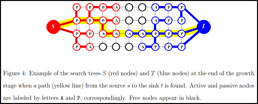
The nodes from either tree can be active or passive. The active nodes $A \subset N$ are the leaves of the tree, while passive nodes are internal. Active nodes $p \in A$ allow the tree to grow by recruiting new children $q$ such that $q \in F$ and $e = (p, q), w_e > 0$. During this process, a $path_{ST}$ is found when a leaf from $S_t$ tries to recruit a leaf from $T_t$ or viceversa. These concepts are schematized by [2] in the following way:
A final subset of nodes $O$ denominated orphans is also considered. The BK algorithm is started by representing the image as a graph, then initializing the search related subsets as $$S_t = Obj, \quad T_t = Bkg, \quad A = Borders(S_t) \cup Borders(T_t), \quad O = \emptyset$$ Some other terms are also defined, namely:
- $TREE(p)$, a flag that stores whether a node is part of $S_t$, $T_t$ or $F$
- $PARENT(p)$, to refer to the parent of $p$ in $TREE(p)$
- $ORIGIN(p)$, which can be either $S$ or $T$ and requires a valid path between $p$ and its respective terminal, otherwise $ORIGIN(p) = \varnothing$
- $cap(p \to q)$, which refers to the residual capacity of the edge $(p, q)$ if $TREE(p) = S_t$ or $(q, p)$ if $TREE(p) = T_t$
After initialization, the algorithm iteratively repeats three stages: Growth, Augmentation and Adoption. Exiting from the loop is controlled by the result of the growth stage.
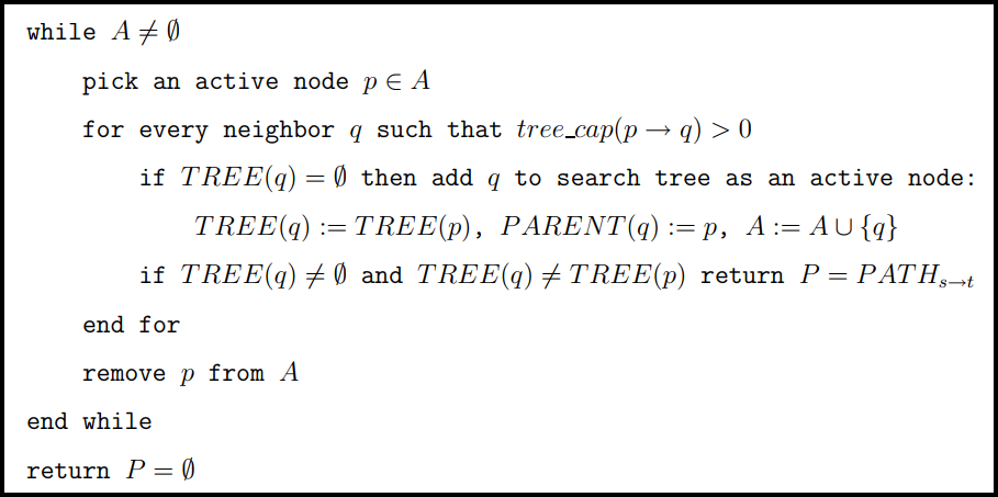
Growth
This stage is summarized by [2] as: "search trees [$S_t$] and [$T_t$] grow until they touch giving a [$path_{ST}$]". This is the stage where active nodes try to recruit new free nodes, until all active nodes are depleted. It returns a $path_{ST}$ if it finds one, otherwise the stage loop ends and $path_{ST}$ is returned as $\emptyset$. This halts the BK algorithm main loop, indicating that the optimal cut was found.
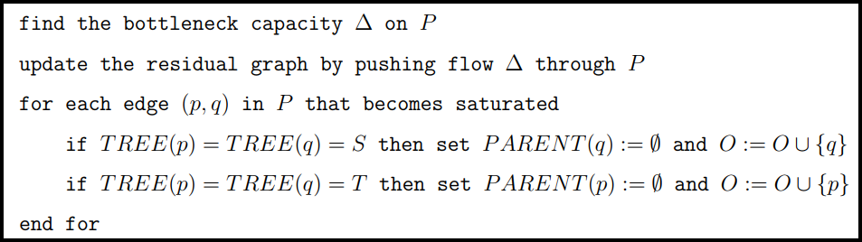
Augmentation
This stage is summarized by [2] as: "the found path is augmented, search tree(s) break into forest(s)". It takes as input the $path_{ST}$ found in the growth stage, and pushes the maximum amount of flow that path can handle. This means one or more edges in the path get saturated, making these edges invalid as a parent-child relationship. An affected child node becomes both an orphan and the root of a new subtree $O_t$ spanning the orphan's descendants. Futhermore, $ORIGIN(n) = \varnothing \quad \forall n \in O_t$.
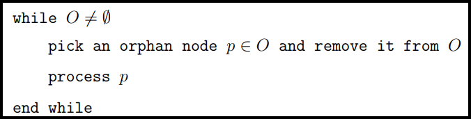
Adoption
This stage is summarized by [2] as: "trees [$S_t$] and [$T_t$] are restored". This stage seeks to find a new valid parent $p$ for each orphan $o$. A valid parent should satisfy $TREE(p) = TREE(o), ORIGIN(p) = TREE(o)$ and the edge connecting them must satisfy $w_e > 0$. If a parent is found, the subtree $O_t$ is restored to the main tree and $ORIGIN(n) = TREE(p) \quad \forall n \in O_t$. If no parent is found, $TREE(o) := F$ and its children are declared as orphans. Furthermore, all neighbours $q$ of $o$ such that $TREE(q) = TREE(o)$ should become active. This procedure is repeated until no orphans are left.
Python Implementation
Requirements
This implementation is written for Python 3.8 and above. It aims to be highly portable, so it has few basic dependencies:
- NumPy for representing images as matrices and optimizing some steps.
- Matplotlib (>= 3.5.0) for building the interactive GUI.
- Pillow for easily handling I/O image operations.
- psutil for benchmarking the amount of memory required by the program.
Basic Usage
The source code of this implementation is available to download here. Downloading src/ is sufficient to execute the implementation, while additional test images can be downloaded from samples/. The source code of this report is also available in docs/.
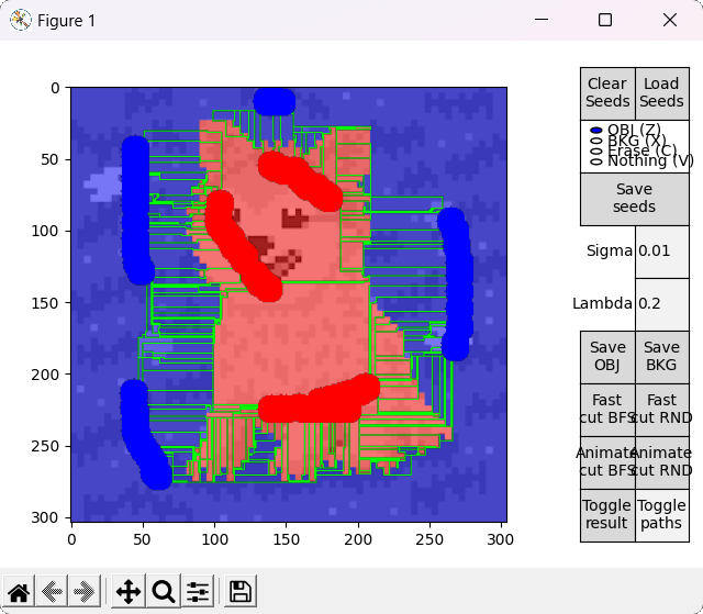
Two scripts are provided as an entry point to the program, GUI_main.py and GUI_details.py. Both of them behave almost identically (the latter displays an additional window with more details of the BK result), so the focus here is on GUI_main.py. When executed, the user is prompted with a window to select an image file. After that, the main window is displayed. To the left, the selected image is displayed in a black and white representation, while to the right different controls are available.
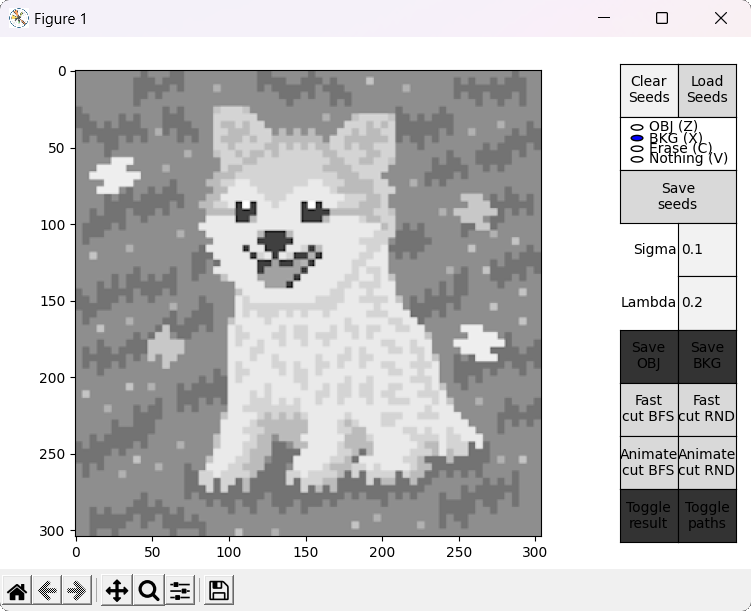
When hovering over the displayed image, four different actions are available. They can be selected by clicking the respective buttons at the right side, or by pressing the specified keyboard shortcut.
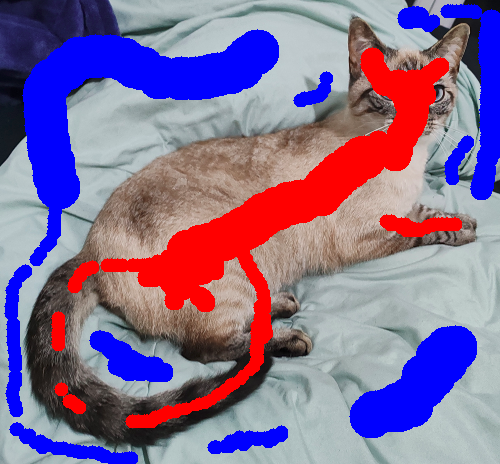
- OBJ allows to draw seeds for the object (shortcut: Z).
- BKG allows to draw seeds for the background (shortcut: X).
- Erase allows to erase any seed (shortuct: C).
- Nothing allows to interact with the standard matplotlib mouse callbacks, e.g. zooming the image (shortcut: V).
Fast and Animate cut modes
After preparing the seeds, the default $\sigma$ and $\lambda$ parameters can be modified. The segmentation can then be initialized, with four different options provided by the interface. Options denominated Fast follow a standard implementation of the BK algorithm's loop, and is to be used when only the result is of interest.
Once the segmentation is obtained, the result is portrayed on top of the displayed image. This representation can be toggled on or off, while the result itself can be saved as an image, either just the object (Save OBJ) or just the background (Save BKG). Note that the algorithm yields a mask, which is used to save a segmentation of the original image and not its black and white representation.

Options denominated Animate follow a slightly different BK algorithm's main loop. The loop performs a fixed amount of iterations, controlled by the parameter CYCLES_PER_FRAME. When concluded, the current state of the search trees and the last $path_{ST}$ are taken to draw a frame on top of the displayed image. Immediatly afterwards, a new loop is started resuming the state of the previous loop. This effectively allows to animate the algorithm's progress and better understand the concepts behind its execution.
When the BK algorithm's loop reaches its natural end, the results are displayed as usual. An additional option is present, Toggle paths, that allows to observe all the instances of $path_{ST}$ present in the animation. CYCLES_PER_FRAME should be assigned a sensible value to allow for a faster animation and avoid cluttering when visualizing all paths.

BFS and RND cut modes
In different flow based algorithms (including BK), the search procedure performed when finding paths is commonly a breadth-first search (BFS). However, different search methods can be employed, and in the case of a heuristic algorithm such as BK, this can mean affecting the performance of the procedure in a positive or negative way (although the optimal cut will always be the same).
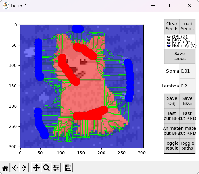
This idea is explored by the options denominated with RND, which employ an alternative version of the BK algorithm that uses a random based search in the growth stage. During this stage, when picking an active node BFS always takes the first node of the ordered array $A$, while RND chooses a node from a different random index each time. For completeness, options denominated with BFS employ the standard BFS based algorithm.
Ideally, in some cases this might allow to find the shortest $path_{ST}$ faster and improve performance, or reduce the number of BK main loop's cycles in some other unforeseen way. However, this is by nature a highly empirical decision. For example, in the images tested for this implementation, RND appears to find some shorter paths than BFS (as observed in the figure below), but ultimately requires slightly more cycles.
Additional Details
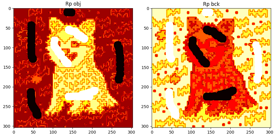
Some additional details can be observed after performing any kind of cut using GUI_details.py. The regional penalties can be observed by plotting the values of the costs of terminal edges. Note that regions of similarly valued edges can be observed around their respective extreme-valued seeds.
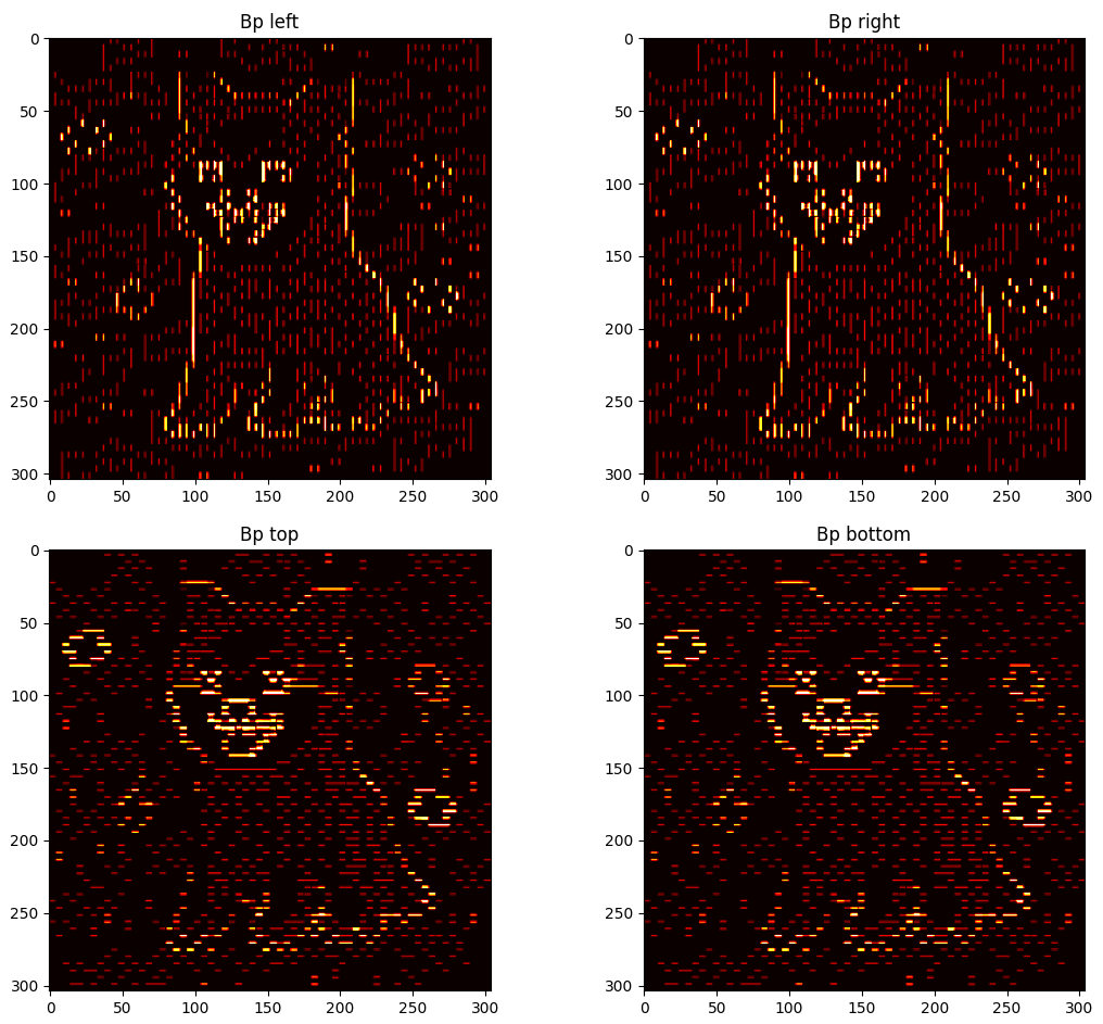
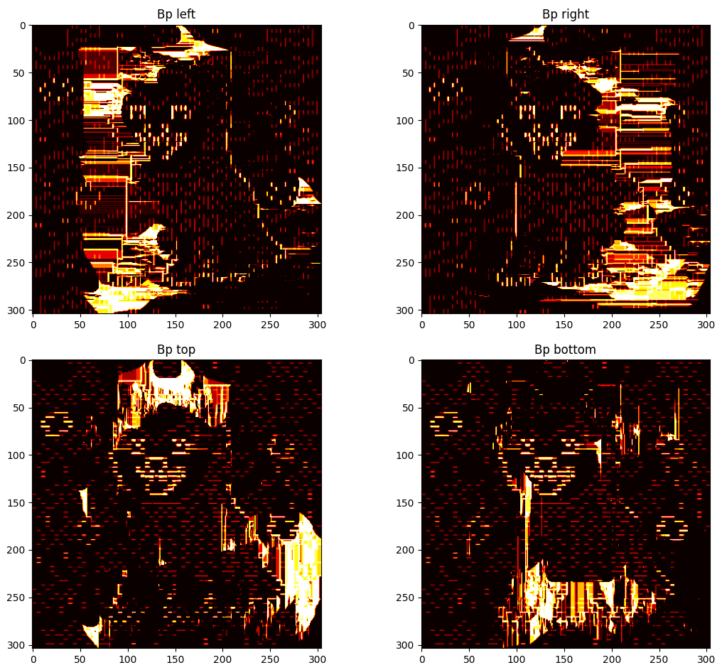
Representing the boundary penalties is a bit trickier. Each pixel is involved in up to four Bp values, one for each direction (left, right, up, down). Therefore, for displaying the values of the costs of non-terminal edges, four different plots are represented, one for each direction.
Note that in the plots for the state before the cut, boundaries of high costs can be observed in sections where there is a drastic change of $Ip$ value. These boundaries are either vertical or horizontal, depending on the direction of the neighbouring relationship. Furthermore, it can be observed that many new perpendicular "borders" are generated after the cut. These are from pixels that belonged to one or more $path_{ST}$ and got saturated through the BK algorithm.
Examples of Usage
Three simple images* with different degrees of complexity were used to test the graph-cut algorithm. The same set of seeds was used for a given image when obtaining different results. Below are some examples of usage under different values of $\sigma$.**
* For this implementation, it is recommended to use images with less than one million pixels to retain performance, specially if performing animations.
** Due to lack of clarity from different sources on how to implement BK, this implementation has a bug where changing $\lambda$ doesn't affect the result. This is to be fixed in the future.


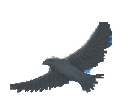
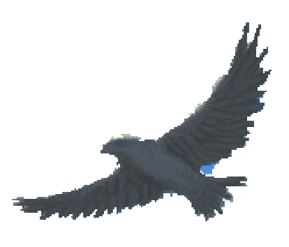


As expected, the results can vary drastically when changing $\sigma$. Reducing it makes the boundary penalty more strict, which can lead to more aggresive cuts and granularity in the results. On the other hand, increasing it relaxes the penalty, which can potentially disrupt how $Bp$ and $Rp$ relate when finding the max-flow and lead to erroneous segmentations.
Nevertheless, if a segmentation is not satisfactory, the seeds or parameters can be adjusted to try and obtain better results. This implementation of the BK algorithm proved to be relatively fast for small images, requiring just a couple of seconds to complete the segmentation and less than 500 MB of memory for the example images, so testing different segmentation settings is indeed viable.
References
- Boykov, Y. Y., and M. P. Jolly. “Interactive Graph Cuts for Optimal Boundary & Region Segmentation of Objects in N-D Images.” Proceedings Eighth IEEE International Conference on Computer Vision. ICCV 2001, vol. 1, 2001, pp. 105–12 vol.1. IEEE Xplore, https://doi.org/10.1109/ICCV.2001.937505. Source.
- Boykov, Y., and V. Kolmogorov. “An Experimental Comparison of Min-Cut/Max- Flow Algorithms for Energy Minimization in Vision.” IEEE Transactions on Pattern Analysis and Machine Intelligence, vol. 26, no. 9, Sept. 2004, pp. 1124–37. DOI.org (Crossref), https://doi.org/10.1109/TPAMI.2004.60. Source.
- Boykov, Yuri, and Gareth Funka-Lea. “Graph Cuts and Efficient N-D Image Segmentation.” International Journal of Computer Vision, vol. 70, no. 2, Nov. 2006, pp. 109–31. Springer Link, https://doi.org/10.1007/s11263-006-7934-5. Source.
- Juan, O., and Y. Boykov. “Active Graph Cuts.” 2006 IEEE Computer Society Conference on Computer Vision and Pattern Recognition (CVPR’06), vol. 1, 2006, pp. 1023–29. IEEE Xplore, https://doi.org/10.1109/CVPR.2006.47. Source.
- Humayun, Ahmad, et al. “RIGOR: Reusing Inference in Graph Cuts for Generating Object Regions.” 2014 IEEE Conference on Computer Vision and Pattern Recognition, 2014, pp. 336–43. IEEE Xplore, https://doi.org/10.1109/CVPR.2014.50. Source.
- The test image "pup.png" was uploaded to a royalty-free hosting website by @thebeekeep. Source.
- The test image "bird.png" was uploaded to a royalty-free hosting website by @Ceru. Source.