Molecular Dynamics

Input preparation

The original PDB files for both mutated and wild types were obtained from the PDB website. The chosen PDB wild-type entry contained an additional ligand, which was manually removed from the file. These two PDB structures were then given as input to the Input Generator tool from Charmm-gui. This tool produces the input files for the different simulations, namely by:

• Constructing the simulation box.
• Adding water and ions into the system.

The workflow changes slightly at the beginning of the process for each system, as described below.

Step	mt2 input files	mt1 input files	wt2 input files	wt1 input files
1	www.charmm-gui.org $\rightarrow$ Input Generator $\rightarrow$ Solution Builder $\rightarrow$ Download PDB File: 8DFN		www.charmm-gui.org $\rightarrow$ Input Generator $\rightarrow$ Solution Builder $\rightarrow$ Upload PDB File: 7si9_modified.pdb. Select Check/Correct PDB Format
2	Select both PROA and PROB	Select only PROA	Select both PROA and PROB	Select only PROA
3	Select Terminal group patching and Model missing residues (select as well the respective residues to model).
4: Solvator	Waterbox Size Options $\rightarrow$ Specify Waterbox Size $\rightarrow$ X,Y,Z = 105 Add Ions $\rightarrow$ Ion Placing Method: Monte-Carlo Basic Ion Types: NaCl $\rightarrow$ Add Simple Ion Type (Concentration: 0.15, Neutralizing) Remove the default KCl
solvent composition should be:	$101 Na^+$, $93 Cl^-$	$103 Na^+$, $99 Cl^-$	$101 Na^+$, $93 Cl^-$	$102 Na^+$, $99 Cl^-$
5: PBC Setup	Periodic Boundary Condition Options $\rightarrow$ Generate grid information for PME FFT automatically
6: Input Generator	Force Field Options $\rightarrow$ CHARMM36m Input Generation Options $\rightarrow$ GROMACS Dynamics Input Generation Options $\rightarrow$ Temperature 310 K

Molecular Dynamics Simulation

The outcome of the previous step is provided in the repository, separated in 4 folders inside data_md/. The parameters for the following steps are also provided in data_md/_params/. The source files for the following steps can also be found in src_md/. It is required to set this as the current working directory before attempting to execute any of the scripts.

Step 0: Energy Minimization

At this point, the system is complete but the protein is still in a high energy configuration. Hence it is necessary to find the configuration associated to the minimum value of the energy and then let it evolve. This is known as energy minimization. The protein is allowed to explore many configurations to find the one associated to a minimum value of the molecular energy.

Parameters employed:

• Integrator: steepest descent
• Energy minimization threshold: $400$
• Integrator step: $0.01$
• Maximum number of steps: $5000$

For running this step, it's necessary to submit 0_EM.pbs as a job (or run locally an equivalent .sh script) only once.

NVT and NPT equilibration

For further stabilizing the initial state of the system, the next steps consist of finding the volume and the pressure values which correspond to the minimum of the molecular energy of the protein. For running this step, it's necessary to submit 1_NVT_NPT.pbs as a job (or run locally an equivalent .sh script) only once.

NVT

Here, the volume is fixed, and the pressure slightly changes until the minimum energy configuration is found. The value of the pressure which corresponds to the minimum energy configuration will be employed in the following step.

Parameters employed:

• Integrator : molecular dynamics
• Temperature : $310 K$
• Number of steps : $250000$
• Time step : $0.002 ps$

The total time of the molecular dynamics evolution is of $250000 \times 0.002 ps = 0.5 ns$.

NPT

Here, the volume slightly changes, until the configuration which corresponds to the minimum energy is found.

Parameters employed:

• Integrator : molecular dynamics
• Temperature : $310 K$
• Number of steps : $500000$
• Time step : $0.002 ps$

The total time of the molecular dynamics evolution is of $500000 \times 0.002 ps = 1 ns$.

Unrestrained Molecular Dynamics

At this point we can proceed with the unrestrained MD simulation.

Parameters employed:

• Integrator : molecular dynamics
• Temperature : $310 K$
• Number of steps : $150000000$
• Time step : $0.002 ns$

The total time of the molecular dynamics evolution is of $150000000 \times 0.002 ps = 300 ns$. For running this step, a script called 2_MD.sh is provided, which simplifies the process of submitting multiple jobs to the cluster. This script needs to be executed multiple times until the simulations reach the desired amount of steps.

Benchmarking

Given the large amount of integration steps required for this phase, it is pertinent to perform a benchmark to better choose the appropriate amount of computational resources needed (i.e. cores). For this project, the MD simulation was performed on high performance CPUs available in cluster of the university.

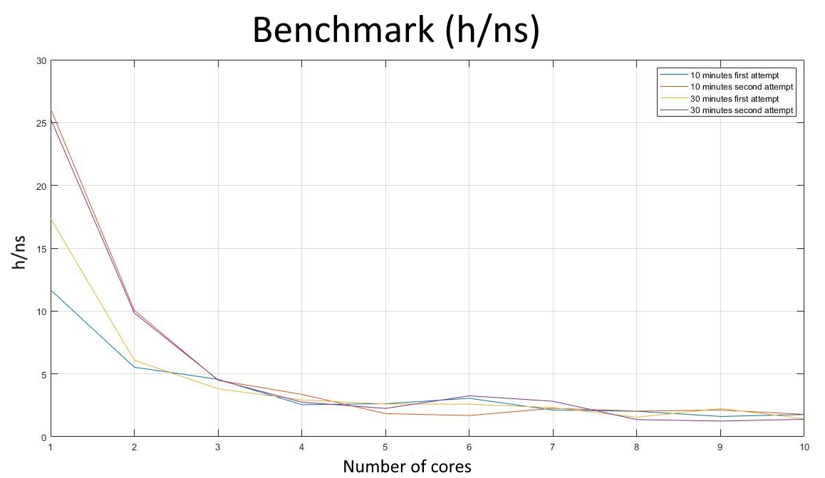
The benchmark process for choosing the right amount of cores is as following. The unrestrained MD was performed with a walltime of $10$ and $30$ minutes. We also repeated the benchmarks two times for each walltime. We noticed that the efficiency obtained with the same number of cores and walltime was not constant. This is probably due to the simulation running on different cores every time, which might have different performances.

In the two plots below it is shown, as an example, the benchmark performed for the NVT equilibration. It can be easily observed that the nanoseconds in the simulation processed in a day, in $ns/day$, and the efficiency, in $h/ns$ (hours to perform a nanosecond of simulation), depend on the wall time. It can be also observed that the outcomes obtained for different repetitions are different.

h/ns ns/day

Post processing

If the resulting md_plain.xtc trajectories are observed, it is evident that they need further processing before analysing them. The script 3_POST.sh is provided to deal with this.

• nojump: First of all, the boundary conditions and the diffusive dynamics are removed, by executing the command echo 1 0 | gmx trjconv -s 4_MD/md_plain.tpr -f 4_MD/md_plain.xtc -o md-nojump.xtc -pbc nojump -center. The piped command echo 1 automatically chooses the protein as centering reference, while echo 0 indicates that the whole system should be centered.
• center: Notably, the solvent molecules diffuse out of the simulation box. To fix this, the command echo 3 0 | gmx trjconv -s 4_MD/md_plain.tpr -f md-nojump.xtc -o md-center.xtc -pbc mol -center is used.
• rottrans: Finally, to stop the protein from rotating during the trajectories, the command echo 1 0 | gmx trjconv -s 4_MD/md_plain.tpr -f md-center.xtc -o md-rottrans.xtc -fit rot+trans is employed. As the protein is being fixed in the center, the box of water molecules adopt the rotation the protein had before, but this behavior will not affect much the subsequent analyses.

plain nojump center rottrans

The aligned trajectories are now ready to be used in the General Analysis.