TD 2

Index

Function Analysis
Intersection of Functions
Problems

Function Analysis

These exercises involve plotting and describing the domain and co-domain of more complex functions. There are different ways of approaching this task, and two of such ideas will be explored here: A top-down approach for exercises "1d" and "1c" and a bottom-up approach for exercise "1g".

Exercise 1d

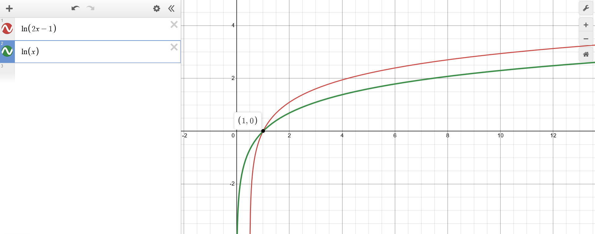
Initially, the behaviour of the function $f(x) = ln(2x-1)$ is unknown. As a starting point, one can think of $f$ as a composition of $g$ and $z$. $$f(x) = g(z(x))$$ In this case, $g(z) = ln(z)$ is the "top-most" function and wraps everything else, which is neatly "packed" in $z(x) = 2x-1$. For the top-down approach, let's first focus on $g(z) = ln(z)$, whose behaviour is well known.

It's known that $g(z) = ln(z)$ intersects with the x-axis at $z_0=1$ and that it has a vertical asymptote at $z^*=0$. Because $g(z)$ is the top-most function, these properties will also be reflected by $f(x)$. One just needs to find the respective values of $x_0$ and $x^*$ where they hold true, which can be achieved by solving $z(x)$ for $z_0$ and $z^*$ respectively. $$\begin{aligned} z(x_0) &= z_0 \\ 2x_0-1 &= 1 \\ x_0 &= 1 \\ \\ z(x^*) &= z^* \\ 2x^*-1 &= 0 \\ x^* &= \frac{1}{2} \\ \end{aligned}$$ Note that these points can also be obtained by considering $z(x)$ as a scaling and shifting operation along the x-axis. This perspective also reveals that $f(x)$ is actually $g(z)$ shrunk by a factor of 2, which wasn't evident before. Knowing this information, one can plot $f(x)$ and find its domain and codomain ($g(z)$ is also shown as reference).

$$\begin{aligned} x &\in (\frac{1}{2}, +\infty) \\ f(x) &\in (-\infty, +\infty) \\ \end{aligned}$$

Exercise 1c

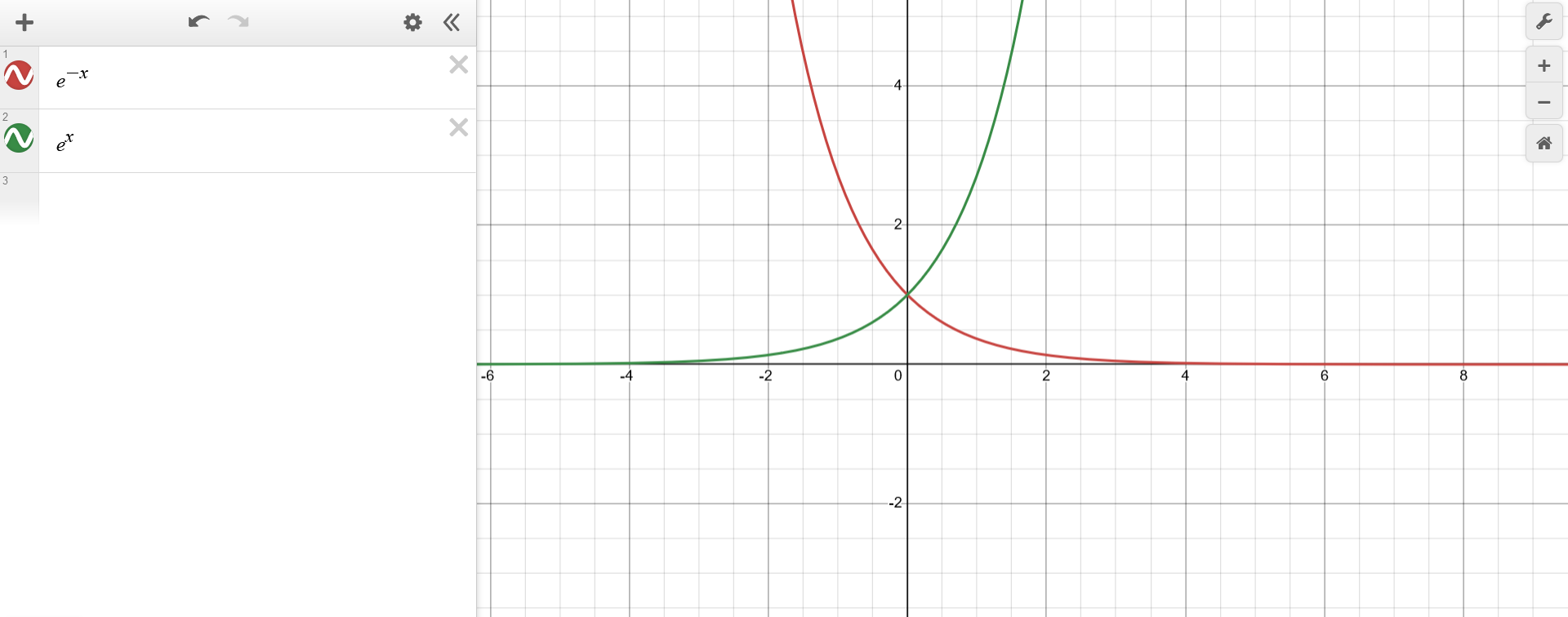
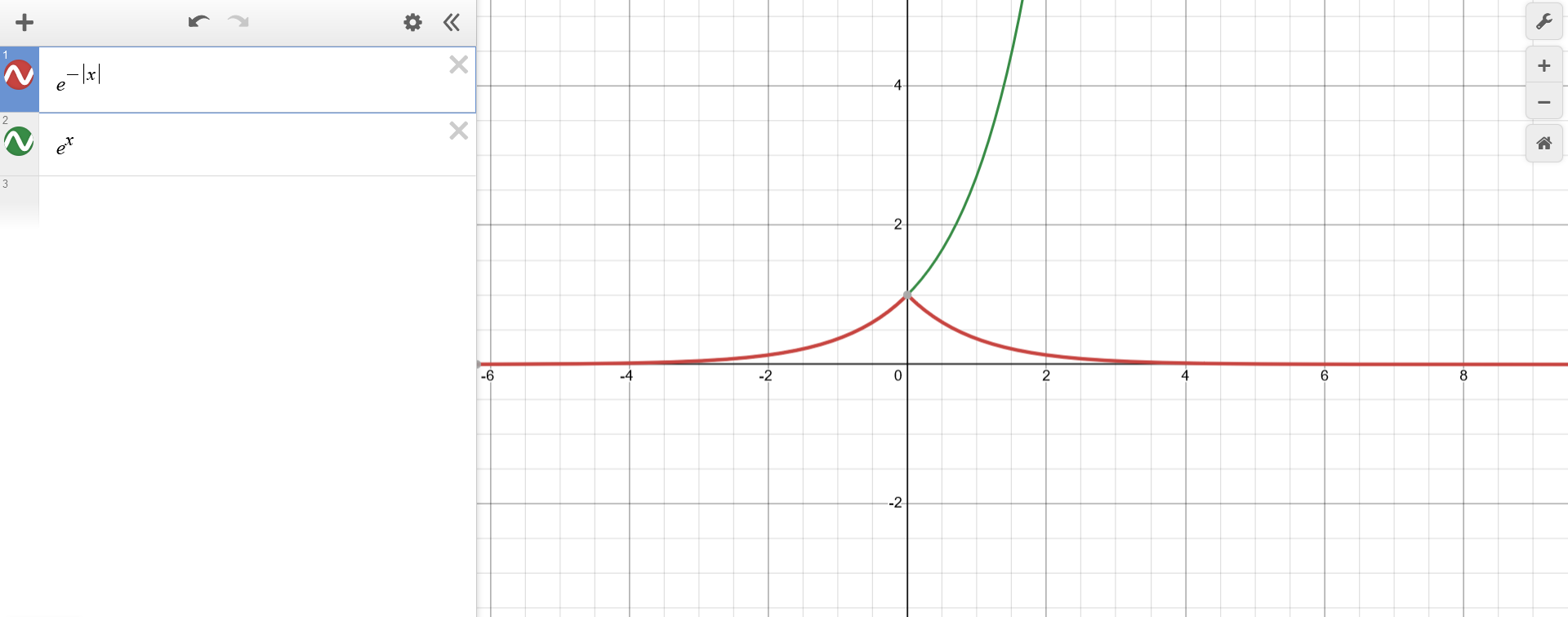
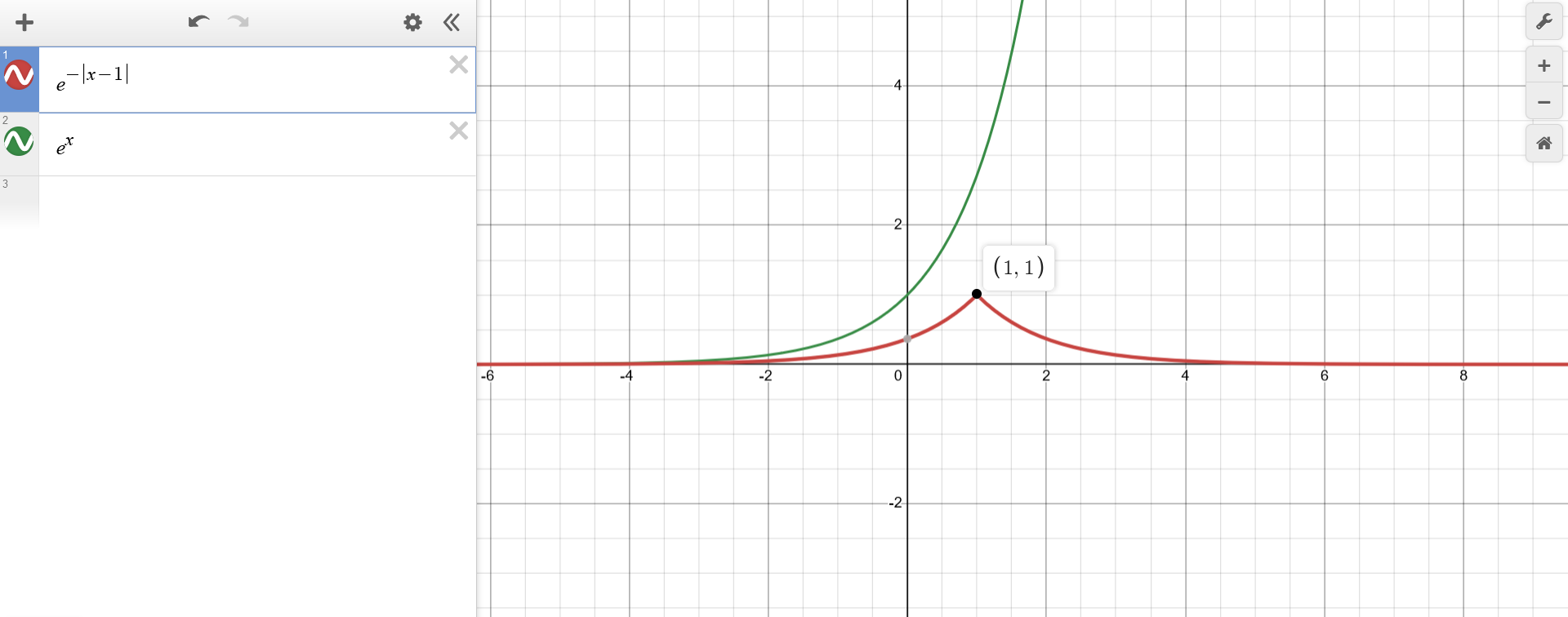
Using the top-down approach, the function $f(x) = e^{-|x-1|}$ can be first represented as $f(x) = a(b(x))$ with $a(b)=e^{-b}$. This means that $a(b)$ is just the well-known exponential function inverted along the x-axis.

Furthermore, the behaviour of $a(b)$ gets affected by the absolute value found in the next "layer" of composition, i.e. $b(c) = |c(x)|$. The effect of the absolute value can be imagined as a "mirror" placed along the y-axis, essentially "reflecting" the values of $b(c > 0)$ into $b(c < 0)$. This behaviour comes from the fact that $|-c(x)|=|c(x)|=c(x)$ and is further propagated to the plot of $a(b(c))$.

Finally, $c(x) = x - 1$ can be considered as a simple shifting operation along the x-axis. This effect is propagated along the chain of function compositions $f(x) = a(b(c(x)))$ by shifting the resulting plot one unit to the right. The final result is the plot for $f(x)$, which also reveals its domain and co-domain.

$$\begin{aligned} x &\in (-\infty, +\infty) \\ f(x) &\in (0,1) \\ \end{aligned}$$

Exercise 1g

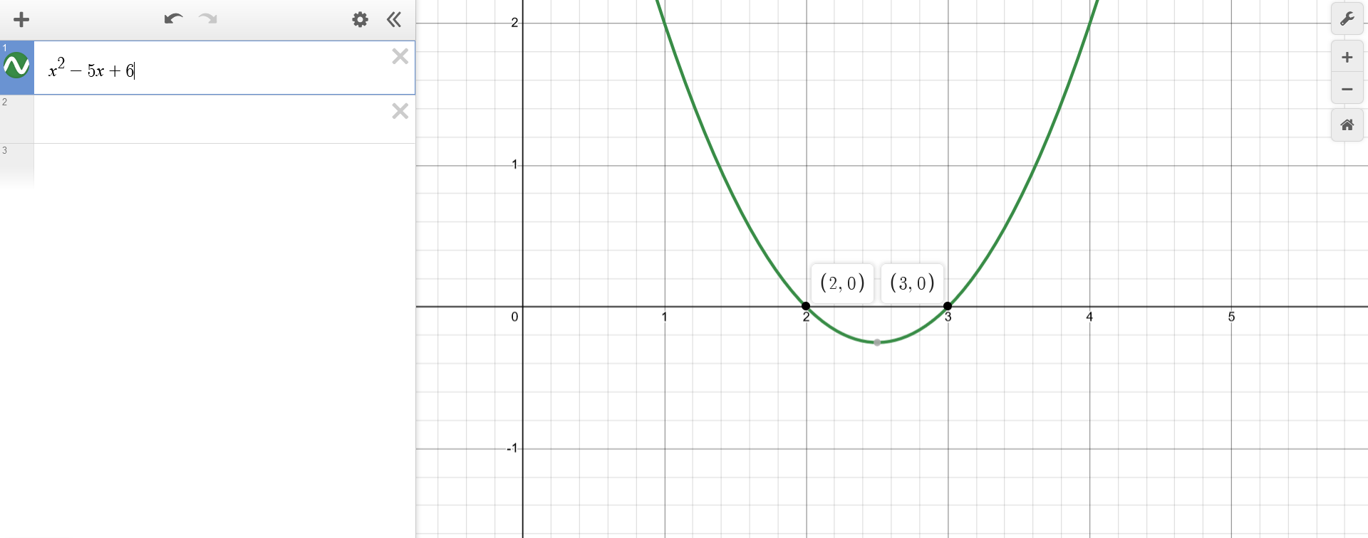
The top-down approach isn't as intuitive for $f(x) = \sqrt{x^2-5x+6}$, so another strategy can be employed. Again, the function can be represented as a composition $f(x) = g(z(x))$, with $g(z) = \sqrt{z}$ and $z(x) = x^2-5x+6$. This time, $z(x)$ will be analyzed first, hence in a bottom-up fashion.
The behaviour of $z(x) = x^2-5x+6$ can be observed by plotting it, which shouldn't be problematic. It is convex (i.e. "looks upwards", as $x^2$ has a positive sign) and it can be factorized as $z(x) = (x-2)(x-3)$, which means it intersects the x-axis at $x=2$ and $x=3$.

Furthermore, the shape and behaviour of the function $g(z) = \sqrt{z}$ is well known.

The idea now is to understand the behaviour of $g(z)$ by exploiting the fact that it's defined in terms of $z$ as its variable. This means that, whenever $z(x)$ grows, $g(z)$ will also grow; note that $g(z)$ "doesn't care" about $x$ in this case. Similarly, whenever $z(x) < 0$, $g(z)$ will be undefined.
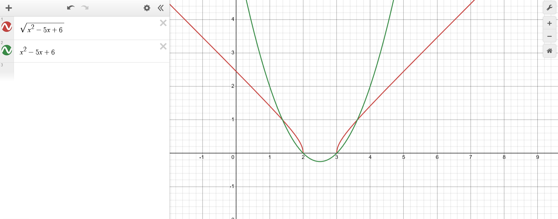
For knowing how to plot $f(x) = g(z)$ at a given point $(x^*,y^*)$, the plot of $z(x) = x^2-5x+6$ becomes handy. One can observe the value at $z^* = z(x^*)$ and use that to know how $y^* = f(z^*)$ should be, following the previous rules. After plotting $f(x)$, the domain and co-domain become once more evident.

$$\begin{aligned} x &\in (-\infty, 2) \cup (3+\infty) \\ f(x) &\in (0,+\infty) \\ \end{aligned}$$

Intersection of Functions

Exercise 2a

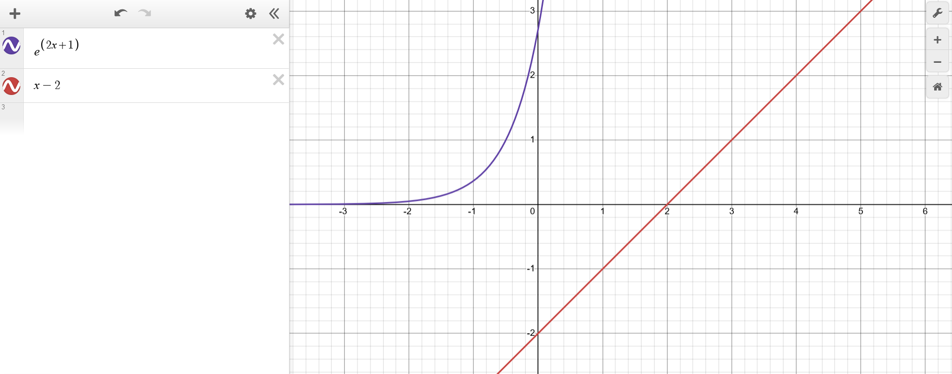
The values of $x$ that comprise the solution for the equation $e^{2x+1}=x-2$ can be inferred by plotting the functions $f(x) = e^{2x+1}$ and $g(x) = x-2$ and finding their point of intersection. After all, when two functions intersect at a given value of $x$, it means that they are equal, which is just a way of rephrasing the original problem.
In this case, one can see that $f(x) = e^{2x+1}$ is simply the exponential function shrunk by a factor of two and shifted horizontally one unit to the left. On the other hand, $g(x) = x-2$ is a simple line shifted two units down. Just by looking at $f(0)=e$ and $g(0)=-2$ and the general shape of these functions, one can plot them and see that, indeed, they do not intersect i.e. there's no solution for $e^{2x+1}=x-2$.

Problems

Exercise 3

The problem is introduced as:

In a chemical reaction, when reactants $A$ and $B$ are mixed, a species $E$ is produced. The amount of species produced depends on the amount of reactant $A$ according to the following law : $q(A) = 2ln(3A+3)$ (...) $E$ depends on $B$ linearly with a proportionality constant of $\frac{1}{2}$.

Knowing this, one can define $E$ as a function of $A$ and $B$, such as $E(A,B)$. For the sake of this example, it will be assumed that the body of $E(A,B)$ simply consists of a product between two terms $q(A)$ and $p(B)$. The body of these two can be taken directly from the quote. $$\begin{aligned} E(A,B) &= q(A)p(B) \\ &= (2ln(3A+3))(\frac{B}{2}) \\ \end{aligned}$$ Now the questions of the problem can be tackled.

How much $E$ will be produced when $A = 1$?

$$\begin{aligned} E(1,B) &= (2ln(3(1)+3))(\frac{B}{2}) \\ &= 2ln(3+3) \frac{B}{2} \\ &= ln(6) B \\ \end{aligned}$$

If we want to double the amount of $E$ produced, what amount of $A$ should be supplied?

Given a fixed value for $A$ and $B$, let lowercase $a$ be the incognita amount required to double $E(A,B)$. $$\begin{aligned} E(a,B) &= 2E(A,B) \\ q(a)q(B) &= 2q(A)q(B) \\ ln(3a+3) &= 2ln(3A+3) \\ ln(3a+3) &= ln((3A+3)^2) \\ 3a+3 &= 9A^2+18A+9 \\ a+1 &= 3A^2+6A+3 \\ a &= 3A^2+6A+2 \\ \end{aligned}$$

Plot the curve of $E$ as a function of $B$.

This is simply the plot for the identity function scaled by a factor of $\frac{1}{2}$.

If we want to double the amount of $E$, how should the amount of $B$ be changed?

Given a fixed value for $A$ and $B$, let lowercase $b$ be the incognita amount required to double $E(A,B)$. $$\begin{aligned} E(A,b) &= 2E(A,B) \\ q(A)q(b) &= 2q(A)q(B) \\ \frac{b}{2} &= 2\frac{B}{2} \\ b &= 2B \\ \end{aligned}$$

Exercise 5

The problem is introduced as:

Two fish populations inhabit the same lake. The population $p_1$ consists of predators that feed on the population $p_2$. The number of fish in each population fluctuates over time according to the predator-prey relationship in a cycle : when the population $p_1$ is low, the population $p_2$ increases, and when the population $p_2$ is large, the population $p_1$ also increases because there is more food ; when the population $p_1$ is large, the population $p_2$ decreases because there are too many predators, and when the population $p_2$ is low, the population $p_1$ decreases as well because there is not enough food. Thus, both populations have a sinusoidal pattern over time.

It states that both $p_1$ and $p_2$ are sinusoidal functions of time, so they could be considered as some variation of $sin(t)$. $$\begin{aligned} p_1(t) &\sim sin(t) \\ p_2(t) &\sim sin(t) \\ \end{aligned}$$

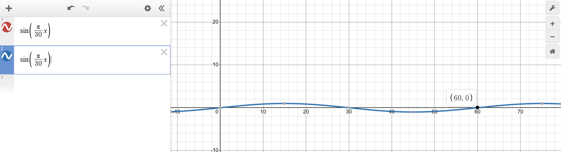
The body of the functions must be improved using further details from the problem, by making use of function manipulation techniques.

The duration of one cycle is 2 months, and there is a phase of 15 days between the phases of the two populations. (...) initially, the population $p_1$ is half that of the population $p_2$.

The first statement hints at a scaling operation over the x-axis: the usual periodicity of $2\pi$ should be converted into $60$ (2 months), by plugging some factor $k$ into $sin(kx)$. Introducing $k=2\pi$ shrinks the periodicity into a value of $\frac{2\pi}{k}=\frac{2\pi}{2\pi}=1$. To extend the periodicity into $60$, $k$ must be further divided by this value. Hence, $k=\frac{2\pi}{60}=\frac{\pi}{30}$. $$\begin{aligned} p_1(t) &\sim sin(\frac{\pi}{30} t) \\ p_2(t) &\sim sin(\frac{\pi}{30} t) \\ \end{aligned}$$

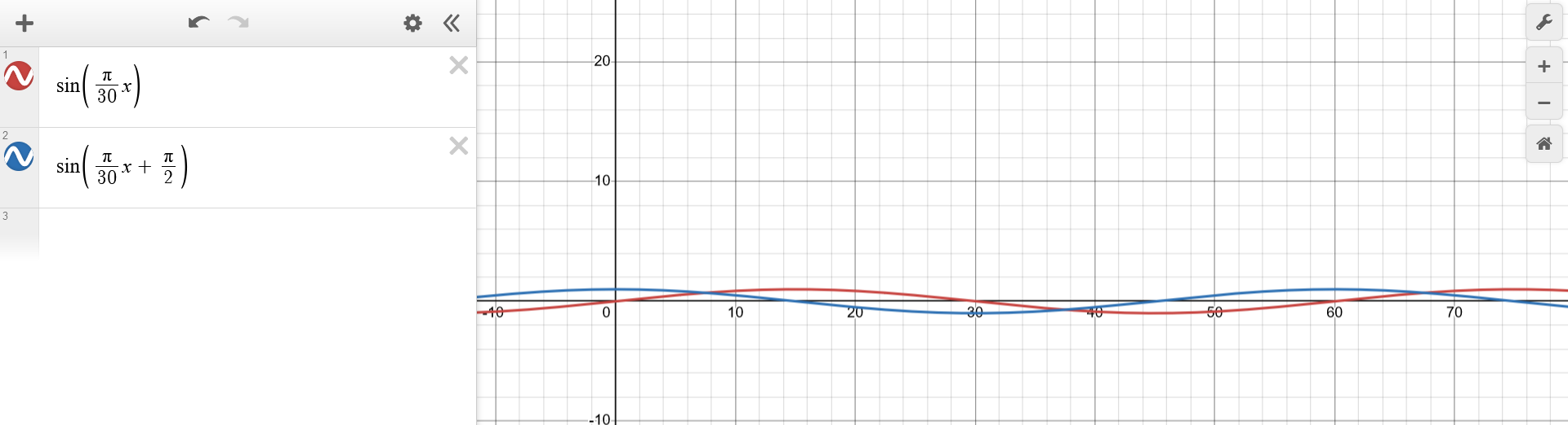
Now, one of the two functions must be shifted horizontally $15$ units, by adding or substracting a factor $c$. Note that $c$ must also be multiplied by $k$, so $c=15k=15\frac{\pi}{30}=\frac{\pi}{2}$. It is stated that $p_1 < p_2$ at $t=0$; one approach is to shift $p_2$ by $15k$ to the left, in order for to shift its previous peak at $t=\frac{k}{2\pi}$ into the new position $t=0$. $$\begin{aligned} p_1(t) &\sim sin(\frac{\pi}{30} t) \\ p_2(t) &\sim sin(\frac{\pi}{30} t + \frac{\pi}{2}) \\ \end{aligned}$$

(...) knowing that the variation in the prey population is twice as large as that for the predators, (...)

The final manipulation directly stated by the problem consists of performing a scaling operation over the y-axis of one of the funtions, by a factor of $2$ (or $\frac{1}{2}$). The intuitive choice is the former. $$\begin{aligned} p_1(t) &\sim sin(\frac{\pi}{30} t) \\ p_2(t) &\sim 2sin(\frac{\pi}{30} t + \frac{\pi}{2}) \\ \end{aligned}$$

Right now, the populations become sometimes negative, which doesn't make physical sense. This can be fixed by shifting both up over the y-axis by some arbitrary amount. Let $b$ be the "base population" of both species, and $a$ the base variation of $p_1$. $$\begin{aligned} p_1(t) &= b + a * sin(\frac{\pi}{30} t) \\ p_2(t) &= b + 2a * sin(\frac{\pi}{30} t + \frac{\pi}{2}) \\ \end{aligned}$$ The fact that $p_2 = 2p_1$ at $t=0$ allows to find a relationship between $a$ and $b$. $$\begin{aligned} p_2(0) &= 2p_1(0) \\ (b + 2a*sin(\frac{\pi}{2})) &= 2(b + a*sin(0)) \\ (b + 2a*1) &= 2(b + a*0) \\ b + 2a &= 2b \\ b &= 2a \\ \end{aligned}$$ For this example, $a$ and $b$ can be set to an arbitrary number, as long as $b = 2a$ holds.

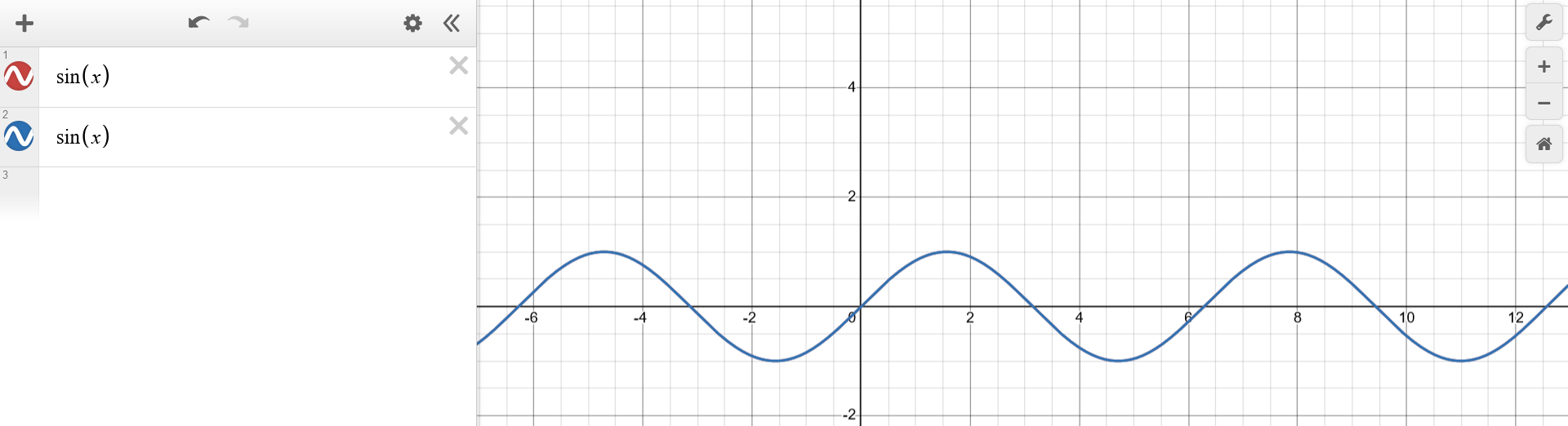
Plot the behavior of both populations on a graph, (...)

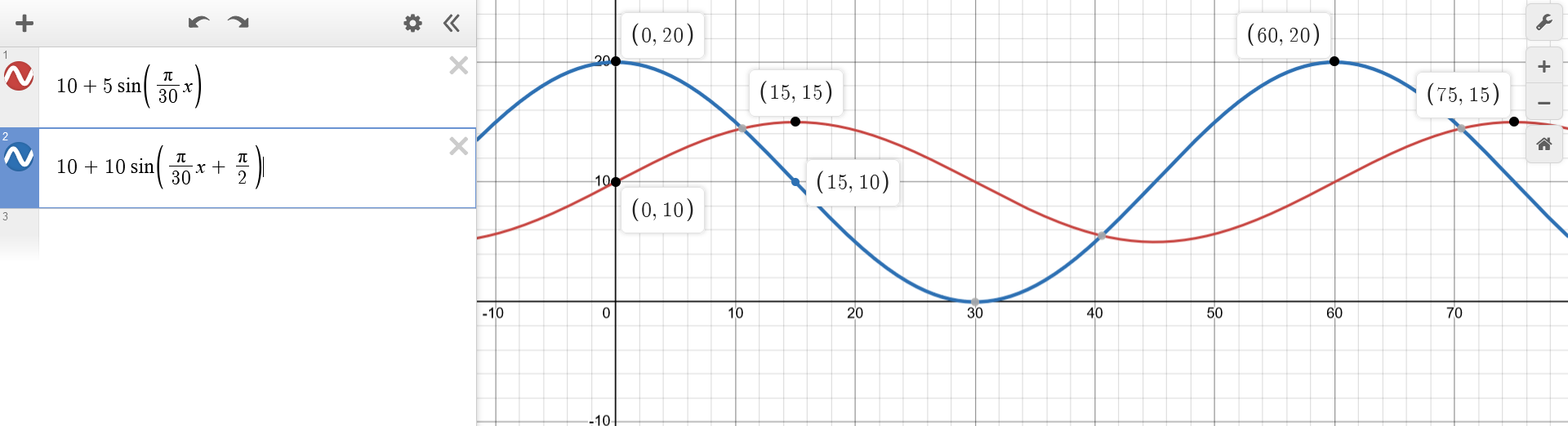
At what point in the cycle are the two populations equal?

The plot shows that $p_1$ and $p_2$ intersect around $t \approx 10.5+30n$ for $n \in \mathbb{N}$. One can solve $p_1(t) = p_2(t)$ for a precise answer. $$\begin{aligned} p_1(t) &= p_2(t) \\ b + a * sin(\frac{\pi}{30} t) &= b + 2a * sin(\frac{\pi}{30} t + \frac{\pi}{2}) \\ sin(\frac{\pi}{30} t) &= 2sin(\frac{\pi}{30} t + \frac{\pi}{2}) \\ sin(\frac{\pi}{30} t) &= 2cos(\frac{\pi}{30} t) \\ tan(\frac{\pi}{30} t) &= 2 \\ \frac{\pi}{30} t &= arctan(2) + n\pi \\ t &= \frac{30}{\pi}(arctan(2) + n\pi) \\ t &= \frac{30}{\pi}arctan(2) + 30n \\ \end{aligned}$$ And indeed $t = \frac{30}{\pi}arctan(2) + 30n \approx 10.572 + 30n$.

When the prey population is at its maximum, what is the population of predators?

The plot immediatly reveals that $p_2(t)$ has maxima at $t = 60n$ and that $p_1(60n) = b$. This can be confirmed by finding the $argmax$ of $p_2(t)$, given the known value of $argmax(sin) = 2\pi n + \frac{\pi}{2}$. Note that the $argmax$ is affected by function manipulations along the x-axis and unaffected by those along the y-axis. The former must be "undone" while the latter can be ignored. $$\begin{aligned} argmax(p_2(t)) &= argmax(b + 2a * sin(\frac{\pi}{30} t + \frac{\pi}{2})) && \\ &= argmax(sin(\frac{\pi}{30} t + \frac{\pi}{2})) && \text{ignore y-axis manipulations} \\ &= \frac{30}{\pi}(argmax(sin(t)) - \frac{\pi}{2}) && \text{"undo" x-axis manipulations} \\ &= \frac{30}{\pi}(2\pi n + \frac{\pi}{2} - \frac{\pi}{2}) && \text{replace known argmax(sin)} \\ &= \frac{30}{\pi}2\pi n && \\ &= 60n && \\ \\ p_1(60n) &= b + a * sin(\frac{\pi}{30} 60n) && \\ &= b + a * sin(2\pi n) && \\ &= b && \\ \end{aligned}$$

How does it change at that moment?

The plot makes evident that $p_1(t)$ increases at $t = 60n$. The derivative $p_1'(t) = \frac{d}{dt} p_1(t)$ indicates how much. $$\begin{aligned} p_1'(t) &= \frac{d}{dt} [b + a * sin(\frac{\pi}{30} t)] \\ &= a*cos(\frac{\pi}{30} t) \frac{d}{dt} [\frac{\pi}{30} t] \\ &= \frac{a \pi}{30} cos(\frac{\pi}{30} t) \\ \\ p_1'(60n) &= \frac{a \pi}{30} cos(\frac{\pi}{30} 60n) \\ &= \frac{a \pi}{30} cos(2\pi n) \\ &= \frac{a \pi}{30} \\ \end{aligned}$$

And when the predator population is at its maximum, what is the population of prey?

Again, the plot reveals that $p_1(t)$ has maxima at $t = 60n + 15$ and that $p_2(60n + 15) = b$ too. This can be confirmed by finding the $argmax$ of $p_1(t)$ in a similar manner as before. $$\begin{aligned} argmax(p_1(t)) &= argmax(b + a * sin(\frac{\pi}{30} t)) && \\ &= argmax(sin(\frac{\pi}{30} t)) && \text{ignore y-axis manipulations} \\ &= \frac{30}{\pi}(argmax(sin(t))) && \text{"undo" x-axis manipulations} \\ &= \frac{30}{\pi}(2\pi n + \frac{\pi}{2}) && \text{replace known argmax(sin)} \\ &= 60n + 15 && \\ \\ p_2(60n + 15) &= b + 2a * sin(\frac{\pi}{30} (60n + 15) + \frac{\pi}{2}) && \\ &= b + 2a * sin(2\pi n + \frac{\pi}{2} + \frac{\pi}{2}) && \\ &= b + 2a * sin(2\pi n + \pi) && \\ &= b && \\ \end{aligned}$$

How does it change at that moment?

The plot makes evident that $p_2(t)$ decreases at $t = 60n + 15$. The derivative $p_2'(t) = \frac{d}{dt} p_2(t)$ indicates how much. $$\begin{aligned} p_2'(t) &= \frac{d}{dt} [b + 2a * sin(\frac{\pi}{30} t + \frac{\pi}{2})] \\ &= \frac{d}{dt} [b + 2a * cos(\frac{\pi}{30} t)] \\ &= -2a*sin(\frac{\pi}{30} t) \frac{d}{dt} [\frac{\pi}{30} t] \\ &= -\frac{a \pi}{15} sin(\frac{\pi}{30} t) \\ \\ p_2'(60n + 15) &= -\frac{a \pi}{15} sin(\frac{\pi}{30} (60n + 15)) \\ &= -\frac{a \pi}{15} sin(2\pi n + \frac{\pi}{2}) \\ &= -\frac{a \pi}{15} cos(2\pi n) \\ &= -\frac{a \pi}{15} \\ \end{aligned}$$